
RELION
RELION developers
Aug 27, 2024

CONTENTS
1 What’s new? 1
1.1 Release 5.0 . . . . . . . . . . . . . . . . . . . . . . . . . . . . . . . . . . . . . . . . . . . . . . . . 1
1.2 Release 4.0 . . . . . . . . . . . . . . . . . . . . . . . . . . . . . . . . . . . . . . . . . . . . . . . . 2
1.3 Release 3.1 . . . . . . . . . . . . . . . . . . . . . . . . . . . . . . . . . . . . . . . . . . . . . . . . 2
2 The team 5
2.1 Current members . . . . . . . . . . . . . . . . . . . . . . . . . . . . . . . . . . . . . . . . . . . . . 5
2.2 Past members . . . . . . . . . . . . . . . . . . . . . . . . . . . . . . . . . . . . . . . . . . . . . . . 6
3 Installation 9
3.1 Download RELION . . . . . . . . . . . . . . . . . . . . . . . . . . . . . . . . . . . . . . . . . . . 10
3.2 Setup a conda environment . . . . . . . . . . . . . . . . . . . . . . . . . . . . . . . . . . . . . . . . 11
3.3 Compilation . . . . . . . . . . . . . . . . . . . . . . . . . . . . . . . . . . . . . . . . . . . . . . . 12
3.4 General configuration . . . . . . . . . . . . . . . . . . . . . . . . . . . . . . . . . . . . . . . . . . 13
3.5 Configuration with CPU acceleration . . . . . . . . . . . . . . . . . . . . . . . . . . . . . . . . . . 14
3.6 Configuration with HIP/ROCm acceleration for AMD GPUs . . . . . . . . . . . . . . . . . . . . . . 15
3.7 Configuration with SYCL acceleration (Intel GPUs) . . . . . . . . . . . . . . . . . . . . . . . . . . 15
3.8 Set-up queue job submission . . . . . . . . . . . . . . . . . . . . . . . . . . . . . . . . . . . . . . . 16
3.9 Edit the environment set-up . . . . . . . . . . . . . . . . . . . . . . . . . . . . . . . . . . . . . . . 17
4 Single particle tutorial 19
4.1 Introduction . . . . . . . . . . . . . . . . . . . . . . . . . . . . . . . . . . . . . . . . . . . . . . . 19
4.2 Preprocessing . . . . . . . . . . . . . . . . . . . . . . . . . . . . . . . . . . . . . . . . . . . . . . . 20
4.3 Particle picking . . . . . . . . . . . . . . . . . . . . . . . . . . . . . . . . . . . . . . . . . . . . . . 27
4.4 Reference-free 2D class averaging . . . . . . . . . . . . . . . . . . . . . . . . . . . . . . . . . . . . 38
4.5 De novo 3D model generation . . . . . . . . . . . . . . . . . . . . . . . . . . . . . . . . . . . . . . 41
4.6 Unsupervised 3D classification . . . . . . . . . . . . . . . . . . . . . . . . . . . . . . . . . . . . . 43
4.7 High-resolution 3D refinement . . . . . . . . . . . . . . . . . . . . . . . . . . . . . . . . . . . . . . 47
4.8 Mask creation & Postprocessing . . . . . . . . . . . . . . . . . . . . . . . . . . . . . . . . . . . . . 50
4.9 CTF and aberration refinement . . . . . . . . . . . . . . . . . . . . . . . . . . . . . . . . . . . . . . 53
4.10 Bayesian polishing . . . . . . . . . . . . . . . . . . . . . . . . . . . . . . . . . . . . . . . . . . . . 56
4.11 Local-resolution estimation . . . . . . . . . . . . . . . . . . . . . . . . . . . . . . . . . . . . . . . 60
4.12 Checking the handedness . . . . . . . . . . . . . . . . . . . . . . . . . . . . . . . . . . . . . . . . . 61
4.13 ModelAngelo: atomic modelling . . . . . . . . . . . . . . . . . . . . . . . . . . . . . . . . . . . . 61
4.14 DynaMight: exploring motions . . . . . . . . . . . . . . . . . . . . . . . . . . . . . . . . . . . . . 63
4.15 Wrapping up . . . . . . . . . . . . . . . . . . . . . . . . . . . . . . . . . . . . . . . . . . . . . . . 66
5 Subtomogram tutorial 69
5.1 Introduction . . . . . . . . . . . . . . . . . . . . . . . . . . . . . . . . . . . . . . . . . . . . . . . 69
5.2 Import . . . . . . . . . . . . . . . . . . . . . . . . . . . . . . . . . . . . . . . . . . . . . . . . . . 70
i

5.3 Motion correction . . . . . . . . . . . . . . . . . . . . . . . . . . . . . . . . . . . . . . . . . . . . 71
5.4 CTF estimation . . . . . . . . . . . . . . . . . . . . . . . . . . . . . . . . . . . . . . . . . . . . . . 73
5.5 Exclude tilt-images . . . . . . . . . . . . . . . . . . . . . . . . . . . . . . . . . . . . . . . . . . . . 75
5.6 Align tilt-series . . . . . . . . . . . . . . . . . . . . . . . . . . . . . . . . . . . . . . . . . . . . . . 76
5.7 Reconstruct tomograms . . . . . . . . . . . . . . . . . . . . . . . . . . . . . . . . . . . . . . . . . 76
5.8 Denoise tomograms . . . . . . . . . . . . . . . . . . . . . . . . . . . . . . . . . . . . . . . . . . . 78
5.9 Particle picking . . . . . . . . . . . . . . . . . . . . . . . . . . . . . . . . . . . . . . . . . . . . . . 79
5.10 Extract subtomos . . . . . . . . . . . . . . . . . . . . . . . . . . . . . . . . . . . . . . . . . . . . . 81
5.11 Import coordinates . . . . . . . . . . . . . . . . . . . . . . . . . . . . . . . . . . . . . . . . . . . . 83
5.12 De novo 3D model generation . . . . . . . . . . . . . . . . . . . . . . . . . . . . . . . . . . . . . . 84
5.13 Reconstruct particle . . . . . . . . . . . . . . . . . . . . . . . . . . . . . . . . . . . . . . . . . . . 86
5.14 Initial 3D refinement . . . . . . . . . . . . . . . . . . . . . . . . . . . . . . . . . . . . . . . . . . . 87
5.15 Duplicate particles removal . . . . . . . . . . . . . . . . . . . . . . . . . . . . . . . . . . . . . . . 92
5.16 3D classification . . . . . . . . . . . . . . . . . . . . . . . . . . . . . . . . . . . . . . . . . . . . . 93
5.17 High-resolution 3D refinement . . . . . . . . . . . . . . . . . . . . . . . . . . . . . . . . . . . . . . 97
5.18 Tomo refinement cycle . . . . . . . . . . . . . . . . . . . . . . . . . . . . . . . . . . . . . . . . . . 100
5.19 Tomo refinement 1: CTF refinement . . . . . . . . . . . . . . . . . . . . . . . . . . . . . . . . . . . 101
5.20 Tomo refinement 2: Bayesian polishing . . . . . . . . . . . . . . . . . . . . . . . . . . . . . . . . . 103
5.21 Model building with ModelAngelo . . . . . . . . . . . . . . . . . . . . . . . . . . . . . . . . . . . 104
6 On-the-fly processing 105
6.1 Computation settings . . . . . . . . . . . . . . . . . . . . . . . . . . . . . . . . . . . . . . . . . . . 105
6.2 Preprocessing settings . . . . . . . . . . . . . . . . . . . . . . . . . . . . . . . . . . . . . . . . . . 106
6.3 Particle settings . . . . . . . . . . . . . . . . . . . . . . . . . . . . . . . . . . . . . . . . . . . . . . 107
6.4 Processing settings . . . . . . . . . . . . . . . . . . . . . . . . . . . . . . . . . . . . . . . . . . . . 107
6.5 Intervening . . . . . . . . . . . . . . . . . . . . . . . . . . . . . . . . . . . . . . . . . . . . . . . . 109
6.6 Control more options . . . . . . . . . . . . . . . . . . . . . . . . . . . . . . . . . . . . . . . . . . . 109
6.7 Site-specific setup . . . . . . . . . . . . . . . . . . . . . . . . . . . . . . . . . . . . . . . . . . . . 110
7 Reference pages 111
7.1 Movie Compression . . . . . . . . . . . . . . . . . . . . . . . . . . . . . . . . . . . . . . . . . . . 111
7.2 Pixel size issues . . . . . . . . . . . . . . . . . . . . . . . . . . . . . . . . . . . . . . . . . . . . . 120
7.3 Automation: Schemes . . . . . . . . . . . . . . . . . . . . . . . . . . . . . . . . . . . . . . . . . . 127
7.4 Helical reconstruction . . . . . . . . . . . . . . . . . . . . . . . . . . . . . . . . . . . . . . . . . . 132
7.5 Subtomogram Averaging . . . . . . . . . . . . . . . . . . . . . . . . . . . . . . . . . . . . . . . . . 133
7.6 Using RELION . . . . . . . . . . . . . . . . . . . . . . . . . . . . . . . . . . . . . . . . . . . . . . 149
7.7 Conventions . . . . . . . . . . . . . . . . . . . . . . . . . . . . . . . . . . . . . . . . . . . . . . . 154
7.8 Developer Guide . . . . . . . . . . . . . . . . . . . . . . . . . . . . . . . . . . . . . . . . . . . . . 158
7.9 Bibliography . . . . . . . . . . . . . . . . . . . . . . . . . . . . . . . . . . . . . . . . . . . . . . . 161
Bibliography 163
ii

CHAPTER
ONE
WHAT’S NEW?
1.1 Release 5.0
Blush regularisation
Dari Kimanius has developed a new method to incorporate more prior knowledge into the cryo-EM refinement process
than the one typically used (which merely assumes smoothness in real-space, or limited power in Fourier-space). This
method is called Blush regularisation and it uses a denoising convolutional neural network inside the iterative refinement
algorithm of Class3D, Refine3D or MultiBody jobs. The effects of this are largest when the signal is weak and standard
refinement in RELION would overfit (as for example visible from streaky artefacts in the solvent region). Using Blush
reglarisation, Dari successfully refined a data set of a 40 kDa protein:RNA complex to 2.5A. The same data set was
intractable in standard RELION or CryoSPARC.
DynaMight for modelling continuous structural heterogeneity
Johannes Schwab developed a method called DynaMight that ‘explores protein Dyna-mics, and Might improve your
map’. It is based on a variational auto-encoder that predicts 3D deformations of a Gaussian model for the consensus
map, and a deformed backprojection algorithm that attempts to “un-do” these deformations to reconstruct an improved
consensus map.
ModelAngelo for automated atomic model building
Kiarash Jamali developed a machine-learning approach for automated atomic model building and identification of
unknown proteins in cryo-EM maps. ModelAngelo will build most of your automatically, provided the resolution
extends beyond 3.5-4.0 Angstroms. Goodbye to months in the dark graphics room!
Select subsets of filaments using dendrograms
David Li developed a useful utility to select subsets of filament particles that belong to the same structural class. It has
been implemented on the Helix tab of the Subset selection job type.
Support for AMD and Intel GPUs (HIP/ROCm and SYCL)
Suyash Tandon from AMD and Jason Do from Intel, together with their colleagues, have contributed code for GPU
acceleration of relion-5 in HIP/ROCm and SYCL, respectively. This means that the relion_refine program can
now also be run efficiently on AMD and Intel GPUs. (The previously existing CUDA implementation and vectorised
CPU-acceleration still work too.)
A complete subtomo-gram averaging pipeline
Alister Burt, Euan Pyle, Sjors Scheres and others have developed a new pipeline for sub-tomogram averaging that starts
with serialEM mdoc files and raw movies, and potentially ends with automated model building by ModelAngelo. You
can access it by launching relion --tomo from the command line. However, please do note that this part of the code
is not yet well tested and we have not yet been able to write an explanatory tutorial for this, so please be patient. Until
we have finished the documentation and testing, you can play with the code already, but we cannot yet provide any
feedback...
1

RELION
1.2 Release 4.0
Watch Sjors giving a Structural Studies Colloquium at MRC-LMB about the new features in release 4.0 on YouTube.
Note that since then, Schedules have been renamed to Schemes to prevent confusion with the existing functionality to
schedule jobs in the GUI.
A new approach to subtomogram averaging
Jasenko Zivanov and Joaquin (Kino) Oton have implemented a new approach to averaging in cryo-electron tomography,
which replaces standard sub-tomograms with the concept of pseudo-sub-tomograms. The new approach leads to better
weighting of the individual 2D images that make up a tilt series in relion_refine and the single-particle concepts of
Bayesian polishing and CTF refinement have now also been implemented for tomography data. A preprint/publication
about this work is pending.
The VDAM refinement algorithm
Dari Kimanius has implemented a new, gradient-driven algorithm with implicit regularisation, called Variable-metric
Gradient Descent with Adaptive Moments (VDAM). The VDAM algorithm replaces the previously implemented SAGD
algorithm for initial model generation, and makes 2D and 3D classification faster, especially for large data sets. A
preprint/publication about this work, together with the automated class selection and the execution of workflow, is
pending.
Automated 2D class selection
Liyi Dong developed a new algorithm for automatic selection of 2D class average images that combines features that
are extracted from RELION’s 2D classification metadata with a convolutional neural network that acts on the 2D class
averages themselves. The corresponding program, relion_class_ranker can be called through the Subset selection
job type.
Automatic execution of workflows
Sjors developed a framework for the automated execution of predefined workflows, which is explained in more detail
in the section on On-the-fly processing.
Tighter integration of the pipeliner with CCP-EM software
The CCP-EM team, mainly Matt Iadanza, Colin Palmer and Tom Burnley, have implemented a python-based pipeliner
in the CCP-EM software that mimics the relion pipeliner, but will be extended to include other CCP-EM softwares
too. The python interface is convenient for scripting, and can also be called from relion’s main GUI, by adding the
additional argument relion --ccpem &.
1.3 Release 3.1
Aberration corrections and optics groups
One of the major new features in relion-3.1 is a correction for higher-order aberrations in the data, i.e. besides the
beamtilt correction already present in relion-3.0, the current version can also estimate and correct for trefoil and tetrafoil,
as well as deviations from the nominal spherical aberration (Cs). The corresponding paper can be found on bioRxiv
[ZNS20]. The signal to estimate these aberrations is calculated by averaging over particles from multiple micrographs.
To allow for multiple subsets of a data set having different Zernike coefficients, relion-3.1 implements the new concept
of optics groups. Optics groups are defined in a separate table called data_optics at the top of a STAR file, which
will also contain a table called data_movies, data_micrographs or data_particles, depending on what type of
images it refers to. The second table is similar to the content of STAR files in previous releases, but contains a new
column called rlnOpticsGroup, which is also present in the data_optics table. Common CTF-parameters, like
rlnVoltage and _`rlnSphericalAberration, but also the new rlnOddZernike and rlnEvenZernike, can be
stored once for each optics group in the data_optics table, without the need to store them for each particle/micrograph
in the second table.
2 Chapter 1. What’s new?
RELION
The same program that handles higher-order aberrations can also be used to refine differences in (anisotropic) mag-
nification between the reference and (groups of) the particles. Besides correcting for anisotropic magnification in the
data, this is also useful when combining data from different scopes. As of release 3.1, the program that does 2D/3D
classification and 3D refinement (relion_refine) can combine particles with different box sizes and pixel sizes in a
single refinement, and the magnification refinement can be used to correct small errors in the (calibrated) pixel sizes.
The box and pixel size of the input reference (or the first optics group in 2D classification) will be used for the re-
constructions/class averages. You may want to check they are on the desired scale before running classifications or
refinements!
Upon reading STAR files that were generated in older releases of relion, relion-3.1 will attempt to convert these auto-
matically into the relion-3.1-style STAR files. Therefore, moving a project from an older release to relion-3.1 should
be easy.
The External job-type
relion-3.1 allows execution of third-party software within the relion pipeline through the new External
job-type. See
this section for details on how to use this.
*Schedules* for on-the-fly processing
The python script relion_it.py in relion-3.0 has been replaced by a new framework of Schedules, which implement
decision-based scheduling and execution of relion jobs. This comes with its own GUI interface. See Schedules for
details on how to use this.
General tweaks
Several tweaks have been made to enhance user experience:
• The pipeliner no longer looks for output files to see whether a job has finished. Instead, upon successful exit, all
programs that are launched from within the relion pipeline will write out a file called RELION_EXIT_SUCCESS
in the job directory. This avoids problems with subsequent execution of scheduled jobs with slow disc I/O.
• Likewise, when encountering an error, all programs will write out a file called RELION_EXIT_FAILURE. The
GUI will recognise these jobs and use a red font in the Finished jobs list. Note that incorrectly labeled jobs can
be changed using the ‘Mask as finished’ or ‘Mark as failed’ options from the Job actions pull-down menu.
• There is an ‘Abort running’ option on the Job actions pull-down menu, which will trigger the currently selected
job to abort. This works because all jobs that are executed from within the relion pipeline will be on the lookout
for a file called RELION_JOB_ABORT_NOW in their output directory. When this file is detected, the job will exit
prematurely and write out a RELION_EXIT_ABORTED file in the job directory. Thereby, users no longer need
to kill undesired processes through the queuing or operating system. The GUI will display aborted jobs with a
strike-through red font in the Finished jobs list.
• When a job execution has given an error, in previous releases the user would need to fix the error through the
input parameters, and then launch a new job. They would then typically delete the old job. relion-3.1 allows to
directly overwrite the old job. This is accessible on Linux systems through ALT+o or through the Overwrite
continue option from the ‘File menu’. Note that the run.out and run.err files will be deleted upon a job
overwrite.
** Tweaks to helical processing **
Several new functionalities were implemented for helical processing:
• The relion_helix_inimodel2d program can be used to generate initial 3D reference maps for helices, in
particular for amyloids, from 2D classes that span an entire cross-over (see this section).
• The translational offsets along the direction of the helical axis can now be restricted to a single rise in 2D-
classification.
1.3. Release 3.1 3

RELION
• The 3D refinement and 3D classification now can use a prior on the first Euler angle, (rlnAngleRotPrior),
which was implemented by Kent Thurber from the Tycko lab at the NIH.
4 Chapter 1. What’s new?

CHAPTER
TWO
THE TEAM
Below are the past and present members of the relion team in reverse chronological order of joining.
2.1 Current members
2.1.1 Bogdan Toader
Google Scholar
Bogdan studied Computer Science and Mathematics at the University of Manchester and did a PhD in Mathematics at
the University of Oxford. He joined the LMB in January 2024 as a postdoc in both our and Tanmay Bharat’s groups to
further improve and develop new tools and algoriths for cryo-ET data processing.
2.1.2 Kiarash Jamali
Google Scholar
Kiarash studied Mathematics and Statistics at the University of Toronto, St George. He joined our group as a PhD
student in October 2021, but had been working with us a volunteering undergrad student since the COVID19 lockdown
in April 2020. Kiarash works on various machine-learning methods for solving cryo-EM structures and beyond.
2.1.3 Johannes Schwab
Google Scholar
Johannes studied Mathematics at the University of Innsbruckm Austria, where he also obtained his PhD. Johannes
works on machine-learning approaches to deal with molecular flexibility in cryo-EM reconstruction.
2.1.4 Dari Kimanius
Google Scholar
Dari studied Theoretical Physics at the Royal Institute of Technology (KTH, Stockholm), and did a PhD in Biophysics
and Bioinformatics at Stockholm University. Dari joined our group as a post-doc in May 2019. Dari implemented
GPU-acceleration during his PhD. For his postdoc at LMB, he works on the incorporation of more informative priors
through deep convolutional neural networks, as well as on the design of more efficient optimisation algorithms.
5

RELION
2.1.5 Euan Pyle
Google Scholar
Euan studied Chemistry and Biology at Durham University before going on to complete his PhD at Imperial College
London. As a post-doc position in Giulia Zanetti’s lab at Birkbeck College/The Francis Crick Institute, he contributed
code to the RELION 5.0 tomography pipeline, in close collaboration with Alister Burt.
2.1.6 Takanori Nakane
Google Scholar
Takanori studied as an M.D. at Kyoto University, where he also obtained his PhD in Medicine. In 2014 he also obtained
an M.Phil in Computational Biology from the University of Cambridge. Takanori joined our team in October 2017. He
works on many facets of single-particle analysis and kindly dedicates a lot of his time to provide support to RELION
users worldwide.
2.1.7 Sjors Scheres
Google Scholar
Sjors studied Chemistry at Utrecht University, The Netherlands, where he also obtained his PhD in protein crystallog-
raphy. He was a post-doc in the group of Jose-Maria Carazo in Madrid, before he started his group at the LMB in 2010.
Sjors designed the regularised likelihood algorithm and is the original architect of relion.
2.2 Past members
2.2.1 Alister Burt
Google Scholar
Alister studied Chemistry at the University at York, UK and did his PhD at the IBS in Grenoble, France. He was a
post-doc in the group of David Barford, where he contributed code to the new sub-tomogram avaraging pipeline in
relion-5;
2.2.2 David Li
Google Scholar
David studied Electrical Engineering and Computer Science at MIT. He worked in the lab of Prof Feng Zhang on
CRISPR systems. David joined our group as an MPhil student in October 2022 to work on in vitro assembly of tau
filaments. During his stay with us David also developed new classification software for filaments. David went on to do
a PhD at Stanford.
6 Chapter 2. The team

RELION
2.2.3 Liyi Dong
Liyi studied Biology at China Agricultural University and did a BSc at Purdue University with Michael Rossmann.
Liyi joined our group as a PhD student in November 2017. She worked on automated selection of 2D class averages.
2.2.4 Shaoda He
Shaoda studied Biology at Peking University, where he also participated in a programme organized by the Electronic
Engineering and Computer Science Department. Shaoda joined our group in October 2014. He developed helical
reconstruction and local symmetry averaging.
2.2.5 Joaquín Otón
Google Scholar
Joaquin (Kino) studied Physics at Universitat de Vàlencia (Spain) and did a PhD in Optical Engineering at Universitat
Politècnica de Catalunya. He joined the neighbouring Briggs group in 2018. Together with Jasenko, he co-developed
a new approach for sub-tomogram averaging.
2.2.6 Jasenko Zivanov
Jasenko studied Computer Science at the University of Basel, Switzerland, where he also obtained his PhD. Jasenko
was a postdoc with us for more than three years (during 2017-2020), and continues to work with us from Switzerland.
Jasenko developed Bayesian polishing and optical aberration correction for single-particle analsyis. Together with
Kino, he also developed a new approach for sub-tomogram averaging.
ò Note
relion is distributed under a GPLv2 license, i.e. it is completely free, open-source software for both academia and
industry.
2.2. Past members 7

RELION
8 Chapter 2. The team

CHAPTER
THREE
INSTALLATION
The sections below explain how to download and install relion on your computer.
Note that relion depends on and uses several external programs and libraries.
C++ compiler:
RELION 5.0 requires a C++ compiler that fully supports the C++14 standard. For GCC, this means version 5.0
or later. Note that GCC 4.8, which comes with RedHat Enterprise Linux / Cent OS 7.x, is too old. You can
obtain newer GCC via devtoolset or use free Intel compiler that comes with oneAPI toolkit (see below).
MPI:
Your system will need MPI runtime (most flavours will do). If you don’t have an MPI installation already on
your system, we recommend installing OpenMPI.
CUDA, HIP/ROCm, SYCL or oneAPI intel compilers:
If you have GPUs from nvidia, AMD or Intel, you can accelerate many jobs considerably.
By default, relion will build with GPU-acceleration support, for which you’ll need cuda. Download it from
NVIDIA website. Note that CUDA toolkits support only a limited range of C compilers. Also note that a newer
CUDA toolkit requires a newer GPU driver. Carefully read the release note and make sure you have a compatible
set of GPU driver, C compiler and CUDA toolkit.
If you want to compile with HIP/ROCm, you will need
• AMD ROCm
If you want to compile with SYCL, you will need
• Intel oneAPI Base Toolkit and HPC Toolkit (All components recommended; this is also recommended
if you want to build the CPU acceleration path, see below)
• Intel software for general purpose GPU capabilities
• Intel CPU Runtime for OpenCL(TM) Applications (optional)
• Codeplay oneAPI for NVIDIA GPU (optional)
• Codeplay oneAPI for AMD GPU (optional)
CTFFIND-4.1:
CTF estimation is not part of relion. Instead, relion provides a wrapper to Alexis Rohou and Niko Grigorieff’s
ctffind 4 [RG15]. Please obtain CTFFIND 4.1.x from their Web site. Note that CTFFIND 5.x is not supported.
Ghostscript:
RELION uses Ghostscript to generate PDF files.
FLTK (only for GUI):
RELION uses FLTK as a GUI tool kit. This will be installed automatically (see below).
9

RELION
X Window system libraries (only for GUI):
RELION needs basic X11 libraries together with Xft for the GUI. Most Linux distributions have packages called
libxft-dev or libXft-devel and libX11-devel. Note that you need developer packages if you build your
own FLTK.
FFT libraries:
RELION needs an FFT library. The default is FFTW. This will be installed automatically (see below). Depending
on your CPU, Intel MKL FFT or AMD optimised FFTW might run faster. See below how to use them.
libtiff:
RELION needs libtiff version >= 4.0. Most Linux distributions have packages called libtiff-dev or
libtiff-devel. Note that you need a developer package.
libpng:
RELION needs libpng. Most Linux distributions have packages called libpng-dev or libpng-devel. Note
that you need a developer package.
pbzip2, xz, zstd:
RELION needs these commands in the PATH to read MRC movies compressed by bzip2, xz or ZStandard, re-
spectively. Note that RELION uses pbzip2, not bzip2. Most Linux distributions provide packages for these
utilities.
UCSF MotionCor2 (optional):
relion implements its own (CPU-only) implementation of the UCSF motioncor2 algorithm for whole-frame mi-
crograph movie-alignment [ZPA+17]. If you want, you can still use the (GPU-accelerated) UCSF program. You
can download it from David Agard’s page and follow his installation instructions. Note that using the UCSF
program does not make full advantage of the opportunities provided in Bayesian polishing.
ResMap (optional):
Local-resolution estimation may be performed inside relion’s own postprocessing program. Alternatively, one
can also use Alp Kucukelbir’s resmap [KST14]. Download it from Alp’s ResMap website and follow his instal-
lation instructions.
In practice, most of these dependencies can be installed by system’s package manager if you have the root priviledge.
In Debian or Ubuntu:
sudo apt install cmake git build-essential mpi-default-bin mpi-default-dev libfftw3-dev␣
˓→libtiff-dev libpng-dev ghostscript libxft-dev
In RHEL, Cent OS, Scientific Linux:
sudo yum install cmake git gcc gcc-c++ openmpi-devel fftw-devel libtiff-devel libpng-
˓→devel ghostscript libXft-devel libX11-devel
3.1 Download RELION
We store the public release versions of relion on GitHub, a site that provides code-development with version control
and issue tracking through the use of git. We will not describe the use of git in general, as you will not need more
than very basic features. Below we outline the few commands needed on a UNIX-system, please refer to general git
descriptions and tutorials to suit your system. To get the code, you clone or download the repository. We recommend
cloning, because it allows you very easily update the code when new versions are released. To do so, use the shell
command-line:
git clone https://github.com/3dem/relion.git
10 Chapter 3. Installation
RELION
This will create a local Git repository. All subsequent git-commands should be run inside this directory.
The master branch (default) contains the stable release of relion-4.0. By performing:
git checkout ver5.0
you can access the latest (developmental) updates for RELION 5.0x.
The code will be intermittently updated to amend issues. To incorporate these changes, use the command-line:
git pull
inside you local repository (the source-code directory downloaded). If you have changed the code in some way, this
will force you to commit a local merge. You are free to do so, but we will assume you have not changed the code.
Refer to external instructions regarding git and merging so-called conflicts if you have changed the code an need to
keep those changes.
3.2 Setup a conda environment
To add support for Python modules (e.g. Blush, ModelAngelo and DynaMight) you will have to setup a Python envi-
ronment with dependencies. We recommend installing via Miniforge to avoid inadvertently installing packages from
the restrictively licensed “default” conda repository.
Once you have conda setup, you can install all the RELION Python dependencies into a new environment by running:
conda env create -f environment.yml
Also code in this environment will be updated intermittently. You can incorporate the latest changes by running:
conda env update -f environment.yml
. Warning
You should NOT activate this relion-5.0 conda environment when compiling and using RELION; RELION
activates it automatically only when necessary. Otherwise, system-wide installation of compilers/libraries/MPI
runtime might get mixed up with those provided by conda, leading to compilation failures or runtime errors. The
same applies to other software packages that provide their own libraries/MPI runtime, such as CCPEM, CCP4,
EMAN2, DIALS, PHENIX.
The cmake command should automatically detect the relion-5.0 conda environment created above. If it does not,
you can specify -DPYTHON_EXE_PATH=path/to/your/conda/python. Additionally, if you intend to make use of
automatically downloaded pretrained model weights (used in e.g. Blush, ModelAngelo and class_ranker), it is recom-
mended to explicitly set the destination directory (TORCH_HOME) by including the flag -DTORCH_HOME_PATH=path/
to/torch/home. You have to create this directory before running cmake. Otherwise, it will be downloaded to the
default location (usually ~/.cache/torch).
At the moment, the model weights for Blush are stored on MRC-LMB’s FTP server. If your network blocks FTP, please
follow instructions here.
3.2. Setup a conda environment 11

RELION
3.3 Compilation
relion has an installation procedure which relies on cmake. You will need to have this program installed, but most
UNIX-systems have this by default. You will need to make a build-directory in which the code will be compiled. This
can be placed inside the repository:
cd relion
mkdir build
cd build
You then invoke cmake inside the build-directoy, but point to the source-directoy to configure the installation. This
will not install relion, just configure the build:
cmake ..
The output will notify you of what was detected and what type of build will be installed. Because relion is rich in terms
of the possible configurations, it is important to check this output. For instance:
• The path to the MPI library.
• GPU-capability will only be included if a CUDA SDK is detected. If not, the program will install, but without
support for GPUs.
• The path to the Python interpreter.
• If FFTW is not detected, instructions are included to download and install it in a local directory known to the
relion installation.
• As above, regarding FLTK (required for GUI). If a GUI is not desired, this can be escaped as explained in the
following section.
The MPI library must be the one you intend to use relion with. Compiling relion with one version of MPI and running the
resulting binary with mpirun from another version can cause crash. Note that some software packages (e.g. CCPEM,
crYOLO, EMAN2) come with their own MPI runtime. Sourcing/activating their environment might update PATH and
LD_LIBRARY_PATH environmental variables and put their MPI runtime into the highest priority.
The MPI C++ compiler (mpicxx) and CUDA compiler (nvcc) internally calls a C++ compiler. This must match the
compiler cmake picked up. Otherwise, the compilation might fail at the linking step.
Following the completion of cmake-configuration without errors, make is used to install the program:
make -j N
, where N is the number of processes to use during installation. Using a higher number simply means that it will compile
faster.
Take note of any warnings or errors reported. relion will be installed in the build directory’s sub-directory called bin.
To make the installation system-wide, see below.
Wherever you install relion, make sure your PATH environmental variable points to the directory containing relion
binaries. Launching relion with a path like /path/to/relion is not the right way; this starts the right GUI, but the
GUI might invoke other versions of relion in the PATH.
12 Chapter 3. Installation

RELION
3.4 General configuration
CMake allows configuration of many aspects of the installation, some of which are outlined here. Note that by default,
relion is configured to build with CUA acceleration on NVidia GPUs. Instructions for building with CPU, HIP/Rocm
(AMD) SYCL (Intel et al) acceleration are given in the next section below.
Most options can be set by adding options to the cmake configuration. Under the below subheadings, some example
replacement commands are given to substitute the original configuration command. It is also recommended to clean
or purge your build-directory between builds, since CMake caches some of previous configurations:
cd build
rm -fr *
And of course, any of the below options can be combined.
Omitting the GUI:
cmake -DGUI=OFF .. (default is ON)
With this option, GUI programs (e.g. relion, relion_manualpick, relion_display) are not be built and
FLTK becomes unnecessary.
Using single-precision on the CPU:
cmake -DDoublePrec_CPU=OFF .. (default is ON)
This will reduce (CPU but not GPU) memory consumption to about half. This is useful when memory hungry
tasks such as motion correction and Polishing run out of memory. This is safe in most cases but please use the
default double precision build if CtfRefine produces NaNs.
Using double-precision on the GPU:
cmake -DDoublePrec_GPU=ON .. (default is OFF)
This will slow down GPU-execution considerably, while this does NOT improve the resolution. Thus, this option
is not recommended.
Compiling NVIDIA GPU codes for your architecture:
cmake -DCUDA_ARCH=52 .. (default is 35, meaning compute capability 3.5, which is the lowest supported by
relion)
CUDA-capable NVIDIA devices have a so-called compute capability, which code can be compiled against for
optimal performance. The compute capability of your card can be looked up at the table in NVIDIA website.
WARNING: If you use a wrong number, compilation might succeed but the resulting binary can fail at the
runtime.
Forcing build and use of local FFTW:
cmake -DFORCE_OWN_FFTW=ON ..
This will download, verify and install FFTW during the installation process.
Forcing build and use of AMD optimized FFTW:
cmake -DFORCE_OWN_FFTW=ON -DAMDFFTW=ON ..
This will download, verify and install AMD optimized version of FFTW during the installation process. This is
recommended for AMD CPUs (e.g. Ryzen, Threadripper, EPYC).
Forcing build and use of Intel MKL FFT:
cmake -DMKLFFT=ON ..
This will use FFT library from Intel MKL. In contrast to the FFTW options above, this will not download MKL
automatically. You have to install MKL and set relevants paths (usually by sourcing the mkl_vars.sh script).
3.4. General configuration 13
RELION
Forcing build and use of local FLTK:
cmake -DFORCE_OWN_FLTK=ON ..
This will download, verify and install FLTK during the installation process. If any of these are not detected
during configuration, this will happen automatically anyway, and you should not have to specify the below options
manually.
Specify location of libtiff:
cmake -DTIFF_INCLUDE_DIR=/path/to/include -DTIFF_LIBRARY=/path/to/libtiff.so.5
This option is to use libtiff installed in non-standard location.
Specifying an installation location:
To allow relion a system-wide installation use:
cmake -DCMAKE_INSTALL_PREFIX=/path/to/install/dir/ ..
make -j N
make install
. Warning
Do not specify the build directory itself as CMAKE_INSTALL_PREFIX. This does not work! If you are happy with
binaries in the build directory, leave CMAKE_INSTALL_PREFIX as default and omit the make install step.
3.5 Configuration with CPU acceleration
Enable accelerated CPU code path:
cmake -DALTCPU=ON
Note that this is mutually exclusive with GPU acceleration (-DCUDA=ON). Intel Classic compilers are recom-
mended for this option (see below).
Use Intel compilers:
There are two Intel compilers: Intel Classic compiler and Intel oneAPI DPC++/C++ compiler. They often gen-
erate faster binaries for Intel CPUs, especially when combined with the accelerated CPU code path above. As of
2024 April, the classic compiler generate faster binaries than the DPC++/C++ compiler.
Both compilers used to be available free of chage as part of Intel oneAPI HPC toolkit. Unfortunately, the classic
compiler was removed in the 2024 release and only the DPC++/C++ compiler is currently distributed. (Ap-
parently older versions seem to be available via YUM/APT, but we do not know how long they remain.) We
recommend you to use the classic compiler if you have older oneAPI toolkit installers at hand.
To use Intel Classic compiler, run below after sourcing the initialization script (setvars.sh):
mkdir build-cpu
cd build-cpu
cmake .. -DMKLFFT=ON \
-DCMAKE_C_COMPILER=icc -DCMAKE_CXX_COMPILER=icpc -DMPI_C_COMPILER=mpiicc -DMPI_CXX_
˓→COMPILER=mpiicpc \
-DCMAKE_C_FLAGS="-O3 -ip -g -xCOMMON-AVX512 -restrict " \
-DCMAKE_CXX_FLAGS="-O3 -ip -g -xCOMMON-AVX512 -restrict "
make -j 24
This generates binaries optimized with AVX512 instructions. If your CPU supports only up to AVX256, use
-xCORE-AVX2 instead of -xCOMMON-AVX512.
14 Chapter 3. Installation

RELION
If you do not have Intel Classic compiler, use the DPC++/C++ compiler from the latest oneAPI release. Its
performance is being improved. The cmake line should be:
cmake .. -DMKLFFT=ON \
-DCMAKE_C_COMPILER=icx -DCMAKE_CXX_COMPILER=icpx -DMPI_C_COMPILER=mpiicx -DMPI_CXX_
˓→COMPILER=mpiicpx \
-DCMAKE_C_FLAGS="-O3 -qopenmp-simd -xCORE-AVX512 -qopt-zmm-usage=high -qoverride-
˓→limits " \
-DCMAKE_CXX_FLAGS="-O3 -qopenmp-simd -xCORE-AVX512 -qopt-zmm-usage=high -qoverride-
˓→limits "
If your CPU supports only up to AVX256, use -xCORE-AVX2 instead of -xCORE-AVX512.
If you don’t want to use Intel MPI, change DMPI_C_COMPILER and DMPI_CXX_COMPILER variables accordingly.
For example, to use OpenMPI with Intel Classic compiler, specify mpicc and mpicxx after setting environmen-
tal variables OMPI_CC=icc and OMPI_CXX=icpc. If cmake still picks up Intel MPI, specify MPI_HOME. See
OpenMPI FAQ and FindMPI manual for details.
3.6 Configuration with HIP/ROCm acceleration for AMD GPUs
Enable the accelerated HIP/ROCm code path with:
cmake -DHIP=ON
Note that this is mutually exclusive with other accelerated code paths (e.g. CUDA, ALTCPU and SYCL). On our
system, we build with HIP/ROCm acceleration to use AMD GPUs with the following commands:
export LD_LIBRARY_PATH=/opt/rocm/lib:$LD_LIBRARY_PATH
export PATH=/opt/rocm/:$PATH
export ROCM_PATH=/opt/rocm/
mkdir build-amd
cd build-amd
cmake -DCMAKE_BUILD_TYPE=Release -DHIP=ON -DHIP_ARCH="gfx90a,gfx908" -DFORCE_OWN_FFTW=ON␣
˓→ -DAMDFFTW=on ..
make -j 24
If you get problems finding omp.h, make sure you have openmp-extras-devel installed on your system too.
3.7 Configuration with SYCL acceleration (Intel GPUs)
Enable accelerated the SYCL code path with:
cmake -DSYCL=ON
Note that this is mutually exclusive with other accelerated code paths (e.g. CUDA, ALTCPU and HIP/ROCm). Tech-
nically speaking, you can build SYCL for AMD and NVIDIA GPUs to make a single binary that runs on NVIDIA,
AMD and Intel GPUs, but this is highly experimental and not tested well.
For now, this way of building RELION is explained here:.
3.6. Configuration with HIP/ROCm acceleration for AMD GPUs 15
RELION
3.8 Set-up queue job submission
The GUI allows the user to submit jobs to a job queueing system with a single click. For this to work, a template job
submission script needs to be provided for the queueing system at hand (e.g. TORQUE, PBS, SGE). In this script a set
of strings (variables) in the template script is replaced by the values given in the GUI. The following table contains all
defined variables:
String Variable Meaning
XXXoutfileXXX string The standard output log file RELION GUI displays.
XXXerrfileXXX string The standard error log file RELION GUI displays.
XXXcommandXXX string relion command + arguments
XXXqueueXXX string Name of the queue to submit job to
XXXmpinodesXXX integer The number of MPI processes to use
XXXthreadsXXX integer The number of threads to use on each MPI process
XXXcoresXXX integer The number of MPI processes times the number of threads
XXXdedicatedXXX integer The minimum number of cores on each node (use this to fill entire
nodes)
XXXnodesXXX integer The total number of nodes to be requested
XXXextra1XXX string Installation-specific, see below
XXXextra2XXX string Installation-specific, see below
The XXXcommandXXX variable needs a special care. For non-MPI commands (e.g. relion_refine) not only the
variable but the whole line is replaced. Thus, mpirun XXXcommandXXX will be mpirun relion_refine_mpi for an
MPI job but relion_refine for a non-MPI job. Also note that some jobs consist of multiple lines of commands. See
CCPEM threads (1 and 2) for typical pitfalls.
There are two environment variables that control the use of the entry of the ‘Minimum number of dedicated cores
per node’ on the Running tabs of the GUI: RELION_MINIMUM_DEDICATED sets its default value (1 if not set);
RELION_ALLOW_CHANGE_MINIMUM_DEDICATED sets whether the user will be able to change this entry. At LMB,
we set the default to 24 and do not allow users to change it. In this way, we enforce that our hyper-threaded 12-core
nodes get filled up entirely by individual relion jobs.
By default, the XXXextra1XXX, XXXextra2XXX, ... variables are not used. They provide additional flexibility for
queueing systems that require additional variables. They may be activated by first setting RELION_QSUB_EXTRA_COUNT
to the number of fields you need (e.g. 2) and then setting the RELION_QSUB_EXTRA1, RELION_QSUB_EXTRA2, ...
environment variables, respectively. This will result in extra input fields in the GUI, with the label text being equal to the
value of the environment variable. Likewise, their default values (upon starting the GUI) can be set through environment
variables RELION_QSUB_EXTRA1_DEFAULT, RELION_QSUB_EXTRA2_DEFAULT, etc and their help messages can be set
through environmental variables RELION_QSUB_EXTRA1_HELP, RELION_QSUB_EXTRA2_HELP and so on. But note
that (unlike all other entries in the GUI) the extra values are not remembered from one run to the other.
The template job submission script may be saved in any location. By default, the one used at the LMB is present as
gui/qsub.csh in the relion tar-ball. Upon installation this file is copied to the bin directory. It is convenient for the
user if he does not have to select this file each time he opens the relion GUI in a new directory. Therefore, one may set
the environment variable RELION_QSUB_TEMPLATE to point to the location of the script for the system at hand. This
value will be pre-set as default in the GUI. (Note the user still has the liberty to define and use his own template!)
ò Note
If somehow the job queue submission cannot be set up, relion may still be run in parallel and on a job queueing
system. The GUI comprises a Print command button that prints the entire relion command, including all arguments,
to the screen. Pasting of this command to a job queue submission script, and manual submission of this script may
16 Chapter 3. Installation

RELION
then be used to submit the parallel job to a queueing system.
3.9 Edit the environment set-up
For relion, we source the following C-shell setup in our .cshrc file. You’ll need to change all the paths for your own
system, and translate the script in case you use a bash shell (which uses export instead of setenv etc).
#!/bin/csh -f
# Setup openMPI if not already done so
if ("" == "`echo $path | grep /public/EM/OpenMPI/openmpi/bin`") then
set path=(/public/EM/OpenMPI/openmpi/bin $path)
endif
if ("1" == "$?LD_LIBRARY_PATH") then
if ("$LD_LIBRARY_PATH" !~ */public/EM/OpenMPI/openmpi/lib*) then
setenv LD_LIBRARY_PATH /public/EM/OpenMPI/openmpi/lib:$LD_LIBRARY_PATH
endif
else
setenv LD_LIBRARY_PATH /public/EM/OpenMPI/openmpi/lib
endif
# Setup |RELION| if not already done so
if ("" == "`echo $path | grep /public/EM/RELION/relion/bin`") then
set path=(/public/EM/RELION/relion/bin $path)
endif
if ("1" == "$?LD_LIBRARY_PATH") then
if ("$LD_LIBRARY_PATH" !~ */public/EM/RELION/relion/lib*) then
setenv LD_LIBRARY_PATH /public/EM/RELION/relion/lib:$LD_LIBRARY_PATH
endif
else
setenv LD_LIBRARY_PATH /public/EM/RELION/relion/lib
endif
# CUDA for RELION
setenv PATH /public/EM/CUDA/Cuda11.4/bin:$PATH
setenv LD_LIBRARY_PATH /public/EM/CUDA/Cuda11.4/lib64:$LD_LIBRARY_PATH
setenv CUDA_HOME /public/EM/CUDA/Cuda11.4
# Where is qsub template script stored
setenv RELION_QSUB_TEMPLATE /public/EM/RELION/relion-devel/bin/qsub.csh
# Default PDF viewer
setenv RELION_PDFVIEWER_EXECUTABLE evince
# Default MOTIONCOR2 executable
setenv RELION_MOTIONCOR2_EXECUTABLE /public/EM/MOTIONCOR2/bin/MotionCor2_1.0.4
# Default CTFFIND-4.1+ executable
setenv RELION_CTFFIND_EXECUTABLE /public/EM/ctffind/ctffind.exe
(continues on next page)
3.9. Edit the environment set-up 17

RELION
(continued from previous page)
# Default ResMap executable
setenv RELION_RESMAP_EXECUTABLE /public/EM/ResMap/ResMap-1.1.4-linux64
# Enforce cluster jobs to occupy entire nodes with 24 hyperthreads
setenv RELION_MINIMUM_DEDICATED 24
# Do not allow the user to change the enforcement of entire nodes
setenv RELION_ALLOW_CHANGE_MINIMUM_DEDICATED 0
# Ask for confirmation if users try to submit local jobs with more than 12 MPI nodes
setenv RELION_WARNING_LOCAL_MPI 12
# Other useful variables
# RELION_MPI_RUN: The mpi runtime ('mpirun' by default)
# RELION_QSUB_NRMPI: The default for 'Number of MPI procs'
# RELION_MPI_MAX: The maximum number of MPI processes available from the GUI
# RELION_QSUB_NRTHREADS: The default for 'Number of threads'
# RELION_THREAD_MAX: The maximum number of threads per MPI process available from the GUI
# RELION_QUEUE_USE: The default for 'Submit to queue?'. "yes" or "no".
# RELION_QUEUE_NAME: The default for 'Queue Name"
# RELION_QSUB_COMMAND: The default for 'Queue submit command'
# RELION_MINIMUM_DEDICATED: The default for 'Minimum dedicated cores per node'
# RELION_ALLOW_CHANGE_MINIMUM_DEDICATED: Whether to allow a user to change the 'Minimum␣
˓→dedicated cores per node' field in the GUI
# RELION_SHELL: A shell used to launch CTFFIND in CtfFind jobs ('csh' by default; only␣
˓→available from 3.1)
# RELION_SCRATCH_DIR: The default scratch directory in the GUI
# RELION_STACK_BUFFER: The buffer size used for MRC(S) file I/O, potentially useful on␣
˓→GPFS or Lustre file system. See https://github.com/3dem/relion/pull/783 for details.
18 Chapter 3. Installation
CHAPTER
FOUR
SINGLE PARTICLE TUTORIAL
4.1 Introduction
This tutorial provides an introduction to the use of relion-5.0 for cryo-EM structure determination. This tutorial covers
the entire single-particle analysis workflow in relion-5.0: beam-induced motion-correction, CTF estimation; auto-
mated particle picking; particle extraction; 2D class averaging; automated 2D class selection; VDAM-based initial
model generation; 3D classification; high-resolution 3D refinement (including Blush regularisation); CTF refinement
and higher-order aberration correction; Bayesian polishing to correct for beam-induced motions in the movies; map
sharpening and local-resolution estimation; automated model building with ModelAngelo; and flexibility analysis with
DynaMight. Carefully going through this tutorial should take less than a day (if you have a suitable GPU or if you
follow our precalculated results). After that, you should be able to run relion on your own data.
This tutorial uses a test data set on beta-galactosidase that was kindly given to us by Takayuki Kato from the Namba
group at Osaka university, Japan. It was collected on a JEOL CRYO ARM 200 microscope. The data and our pre-
calculated results may be downloaded and unpacked using the commands below. The full data set is also available at
EMPIAR-10204.
wget ftp://ftp.mrc-lmb.cam.ac.uk/pub/scheres/relion30_tutorial_data.tar
wget ftp://ftp.mrc-lmb.cam.ac.uk/pub/scheres/relion50_tutorial_precalculated_results.tar.
˓→gz
tar -xf relion30_tutorial_data.tar
tar -zxf relion50_tutorial_precalculated_results.tar.gz
If you have any questions about relion, first read this entire document, check the FAQ on the relion Wiki and the archives
of the CCPEM mailing list. If that doesn’t help, subscribe to the CCPEM email list and use the email address above
for asking your question.
³ Caution
Please, please, please, do not send us direct emails, as we can no longer respond to all of those.
19
RELION
4.2 Preprocessing
4.2.1 Getting organised
We recommend to create a single directory per project, i.e. per structure you want to determine. We’ll call this the
project directory. It is important to always launch the RELION graphical user-interface (GUI) from the project
directory. Inside the project directory you should make a separate directory to store all your raw micrographs or
micrograph movies in MRC, TIFF or EER format. We like to call this directory Movies/ if all movies are in one
directory, or for example Movies/15jan16/ and Movies/23jan16/ if they are in different directories (e.g. because
they were collected on different dates). If for some reason you do not want to place your movies inside the relion project
directory, then inside the project directory you can also make a symbolic link to the directory where your movies are
stored.
. Warning
Symbolic links must be made by an absolute path (e.g. /storage/data/15jan16). Use of relative paths (e.g. ..
/../storage/data/15jan16) can cause problems in later steps. Our precalculated example contains a symbolic
link from Movies to ../Tutorial4.0/Movies/ but please do not follow this practice. Because we don’t know where
you decompress the archive, we cannot include a link by an absolute path.
Single-image micrographs should have a .mrc extension, while movies can have a .mrc, .mrcs, .tif, .tiff or .eer
extension. For EER movies, see this for the details. RELION 5.0 can also read MRC movies compressed by bzip2,
xz, zstd or gzip. When you unpacked the tutorial test data, the (Movies/) directory was created. It should contain
24 movies in compressed TIFF format, a gain-reference file (gain.mrc) and a NOTES file with information about the
experiment.
We will start by launching the relion GUI. As said before, this GUI always needs to be launched from the project
directory. To prevent errors with this, the GUI will ask for confirmation the first time you launch it in a new directory.
Make sure you are inside the project directory, and launch the GUI by typing:
relion &
and answer Yes when prompted to set up a new relion project here.
The first thing to do is to import the set of recorded micrograph movies into the pipeline. Select Import from the
job-type browser on the left, and fill in the following parameters on the Movies/mics tab:
Import raw movies/micrographs?
Yes
Raw input files:
Movies/*.tiff
Are these multi-frame movies?
Yes
(Set this to No if these are single-frame micrographs)
Optics group name:
opticsGroup1
(This field can be used to divide the data set into multiple optics groups: separately import each
optics group with its own name, and then use the Join star files jobtype to combine the groups.
MTF of the detector:
mtf_k2_200kV.star
20 Chapter 4. Single particle tutorial

RELION
Pixel size (Angstrom):
0.885
Voltage (kV):
200
Spherical aberration (mm):
1.4
Amplitude contrast:
0.1
Beamtilt in X (mrad):
0
Beamtilt in Y (mrad):
0
The MTF file can be obtained from the Gatan Web site. If you are working offline and cannot obtain the file, you can
ignore it. The MTF correction does not change the final resolution (but changes the B factor). You can also apply it in
PostProcessing.
On the Others tab, make sure the following is set:
Import other node types?
No
You may provide a meaningful alias (for example: movies) for this job in the white field named Current job:
Give_alias_here. Clicking the Run! button will launch the job. A directory called Import/job001/ will be cre-
ated, together with a symbolic link to this directory that is called Import/movies. Inside the newly created directory
a star file with all the movies is created. Have a look at it using:
less Import/job001/movies.star
If you had extracted your particles in a different software package, then instead of going through the Preprocessing
steps below, you would use the same Import job-type to import particles star file, 3D references, 3D masks, etc. Note
that this is NOT the recommended way to run relion, and that the user is responsible for generating correct star files.
4.2.2 Beam-induced motion correction
The Motion correction job-type implements relion’s own (CPU-based) implementation of the UCSF motioncor2 pro-
gram for convenient whole-frame movie alignment, as well as a wrapper to the (GPU-based) motioncor2 program
itself [ZPA+17]. Besides executing the calculations on the CPU/GPU, there are three other differences between the two
implementations:
• Bayesian polishing (for per-particle motion-correction; see this section) can only read local motion tracks from
our own implementation;
• The motioncor2 program performs outlier-pixel detection on-the-fly, and this information is not conveyed to
Bayesian polishing , which may result in unexpectedly bad particles after polishing;
• Our own implementation can write out the sum of power spectra over several movie frames, which can be passed
directly into ctffind 4.1 for faster CTF-estimation.
For these three reasons, we now favour running our own implementation.
On the I/O tab set:
4.2. Preprocessing 21

RELION
Input movies STAR file:
Import/job001/movies.star
(Note that the Browse button will only list movie star files.)
First frame for corrected sum:
1
Last frame for corrected sum:
-1
(This will result in using all movie frames.)
Dose per frame (e/A2)
1.277
Pre-exposure (e/A2)
0
EER fractionation
32
(This option will be ignored for TIFF files.)
Write output in float16?
Yes
(This will save a factor of 2 in disk space compared to the default of writing in float32. Note that RE-
LION and CCPEM will read float16 images, but other programs may not (yet) do so. For example,
Gctf will not work with float16 images. Also note that this option does not work with UCSF Mo-
tionCor2. For CTF estimation, use CTFFIND-4.1 with pre-calculated power spectra, by activating
the ‘Save sum of power spectra’ option below.)
Do dose-weighting?
Yes
Save non-dose-weighted as well?
No
(In some cases non-dose-weighted micrographs give better CTF estimates. To save disk space, we’re
not using this option here as the data are very good anyway.)
Save sum of power spectra?
Yes
Sum of power spectra every e/A2:
4
(This seems to be a good value according to measurements by Greg McMullan and Richard Hender-
son.)
Fill in the Motion tab as follows:
Bfactor:
150
(use larger values for super-resolution movies)
Number of patches X,Y
5 5
22 Chapter 4. Single particle tutorial

RELION
Group frames:
1
Binning factor:
1
(we often use 2 for super-resolution movies)
Gain-reference image:
Movies/gain.mrc
(This can be used to provide a gain-reference file for on-the-fly gain-reference correction. This is
necessary in this case, as these movies are not yet gain-corrected.)
Gain rotation:
No rotation (0)
Gain flip:
No flipping (0)
Defect file:
(This can be used to mask away broken pixels on the detector. Formats supported in our own im-
plementation and in UCSF motioncor2 are either a text file in UCSF motioncor2 format (each line
contains four numbers: x, y, width and height of a defect region); or a defect map (an image in MRC
or TIFF format, where 0=good and 1=bad pixels). The coordinate system is the same as the input
movie before application of binning, rotation and/or flipping. Note that defect text files produced
by SerialEM are NOT supported! However, one can convert a SerialEM-style defect file into a
defect map using imod.)
Use RELION’s own implementation?
Yes
(this reduces the requirement to install the UCSF implementation. If you have the UCSF program
installed anyway, you could also use that one. In that case, you also need to fill in the options below.)
Fill in the Running tab as follows:
Number of MPI procs:
1
(Assuming you’re running this tutorial on a local computer)
Number of threads:
12
(As these movies are 24 frames, each thread will do two movie frames)
Submit to queue?
No
(Again, assuming you’re running this tutorial on a local computer)
Executing this program takes approximately 5 minutes when using 12 threads on a reasonably modern machine. Note
that our own implementation of the motioncor2 algorithm does not use a GPU. This program is multi-threaded. As
each thread will work independently on a movie frame, it is optimal to use a number of threads such that the number of
movie frames divided by the number threads is an integer number. As these movies have 24 frames, using 12 threads
will result in 2 frames being processed by each thread. You can look at the estimated beam-induced shifts, and their
statistics over the entire data set, by selecting the out: logfile.pdf from the Display: button below the run buttons,
or you can look at the summed micrographs by selecting out: corrected_micrographs.star. Depending on the size of
4.2. Preprocessing 23

RELION
your screen, you should probably downscale the micrographs (Scale: 0.3) and use Sigma contrast: 3 and few
columns (something like Number of columns: 3) for convenient visualisation. Note that you cannot select any
micrographs from this display. If you want to exclude micrographs at this point (which we will not do, because they
are all fine), you could use the Subset selection job-type.
4.2.3 CTF estimation
Next, we will estimate the CTF parameters for each corrected micrograph. You can use the CTF estimation job-type
as a wrapper to Alexis Rohou and Niko Grigorieff’s ctffind 4.1 to execute efficiently on the CPU. We now prefer ctffind
4.1, as it is the only open-source option, and because it allows reading in the movie-averaged power spectra calculation
by relion’s own implementation of the motioncor2 algorithm. Support for GCTF was dropped in RELION 5.0. Fill in
the settings as follows:
On the I/O :
Input micrographs STAR file:
Motioncorr/job002/corrected_micrographs.star
(You can again use the Browse button to select the corrected_micrographs.star file of the
Motion correction job.)
Use micrograph without dose-weighting?
No
(These may have better Thon rings than the dose-weighted ones, but we decided in the previous step
not to write these out)
Estimate phase shifts?
No
(This is only useful for phase-plate data)
Amount of astigmatism (A):
100
(Assuming your scope was reasonably well aligned, this value will be suitable for many data sets.)
On the CTFFIND-4.1 tab, set:
Use CTFFIND-4.1?
Yes
CTFFIND-4.1 executable:
/wherever/it/is/ctffind.exe
Use power spectra from MotionCorr job?
Yes
(We can use these, as we told relion’s own implementation of the motioncor2 algorithm to write these
out in the previous section.)
Use exhaustive search?
No
(In difficult cases, the slower exhaustive searches may yield better results. For these data, this is not
necessary.)
Estimate CTF on window size (pix)
-1
24 Chapter 4. Single particle tutorial
RELION
(If a positive value is given, a squared window of this size at the center of the micrograph will be
used to estimate the CTF. This may be useful to exclude parts of the micrograph that are unsuitable
for CTF estimation, e.g. the labels at the edge of photographic film. )
FFT box size (pix):
512
Minimum resolution (A):
30
Maximum resolution (A):
5
Minimum defocus cvalue (A):
5000
Maximum defocus cvalue (A):
50000
Defocus step size (A):
500
On the Running tab, use six MPI processes to process the 24 micrographs in parallel. This took less than 10 seconds on
our machine. Once the job finishes there are additional files for each micrograph inside the output CtfFind/job003/
Movies directory: the .ctf file contains an image in MRC format with the computed power spectrum and the fitted
CTF model; the .log file contains the output from ctffind; the .com file contains the script that was used to launch
ctffind.
You can visualise all the Thon-ring images using the Display button, selecting out: micrographs_ctf.star. The
zeros between the Thon rings in the experimental images should coincide with the ones in the model. Note that you can
sort the display in order of defocus, maximum resolution, figure-of-merit, etc. The logfile.pdf file contains plots of
useful parameters, such as defocus, astigmatism, estimated resolution, etc for all micrographs, and histograms of these
values over the entire data set. Analysing these plots may be useful to spot problems in your data acquisition.
If you see CTF models that are not a satisfactory fit to the experimental Thon rings, you can delete the .log files
for those micrographs, select the CtfFind/job003 entry from the Finished jobs list, alter the parameters in the
parameter-panel, and then re-run the job by clicking the Continue! button. Only those micrographs for which a .log
file does not exist will be re-processed. You can do this until all CTF models are satisfactory. If this is not possible,
or if you decide to discard micrographs because they have unsatisfactory Thon rins, you can use the Subset selection
job-type to do this.
4.2.4 Manual particle picking
The next job-type Manual picking may be used to manually select particle coordinates in the (averaged) micrographs.
We like to manually select at least several micrographs in order to get familiar with our data. Often, the manually
selected particles to calculate reference-free 2D class averages, which will then be used as templates for automated
particle picking of the entire data set. However, as of release 3.0, relion also contains a reference-free auto-picking
procedure based on a Laplacian-of-Gaussian (LoG) filter. In many cases, this procedure provides reasonable starting
coordinates, so that the Manual picking step may be skipped. The pre-shipped Schemes for on-the-fly processing in the
relion_it.py script make use of this functionality to perform fully automated on-the-fly processing. In this tutorial,
we will just launch a Manual picking job for illustrative purposes, and then proceed with LoG-based Auto-picking to
generate the first set of particles.
Picking particles manually is a personal experience! If you don’t like to pick particles in relion, we also support
coordinate file formats for Jude Short’s ximdisp [Smi99] (with any extension); for xmipp-2.4 [SNRS+08] (with any
extension); and for Steven Ludtke’s e2boxer.py [TPB+07] (with a .box extension). If you use any of these, make
4.2. Preprocessing 25

RELION
sure to save the coordinate files as a text file in the same directory as from where you imported the micrographs (or
movies), and with the same micrograph rootname, but a different (suffix+) extension as the micrograph, e.g. Movies/
006.box or Movies/006_pick.star for micrograph Movies/006.mrc. You should then use the Import job-type
and set Node type: to 2D/3D particle coordinates. Make sure that the Input Files: field contains a linux
wildcard, followed by the coordinate-file suffix, e.g. for the examples above you have to give Movies/*.box or
Movies/*_pick.star, respectively.
On the I/O tab of the Manual picking job-type, use the Browse button to select the micrographs_ctf.star file that
was created in CtfFind/job003, ignore the Colors tab, and fill in the Display tab as follows:
Particle diameter (A):
200
(This merely controls the diameter of the circle that is displayed on the micrograph.)
Scale for micrographs:
0.25
(But this depends on your screen size)
Sigma contrast:
3
(Micrographs are often best display with sigma-contrast, i.e. black will be 3 standard deviation
below the mean and white will be 3 standard deviations above the mean. The grey-scale is always
linear from black to white. See the DisplayImages entry on the RELION wiki for more details)
White value:
0
(Use this to manually set which value will be white. For this to work, Sigma contrast should be
set to 0)
Black value:
0
(Use this to manually set which value will be black. For this to work, Sigma contrast should be
set to 0)
Lowpass filter (A):
-1
(Playing with this may help you to see particles better in very noisy micrographs)
Highpass filter (A):
-1
(This is sometimes useful to remove dark->light gradients over the entire micrograph)
Pixel size:
0.885
(This is needed to calculate the particle diameter, and the low- and high-pass filters)
OR use Topaz denoising?:
Yes
(This has been a feature since relion-4.0 and will make a system call to topaz)
26 Chapter 4. Single particle tutorial
RELION
ò Note
As of relion-5.0, Topaz comes pre-installed in the relion-5 conda environment, which should be picked up auto-
matically by the GUI.
Run the job by clicking the Run! button and click on a few particles if you want to. However, as we will use the
LoG-based autopicking in the next section, you do not need to pick any if you don’t want to. If you were going to use
manually picked particles for an initial 2D classification job, then you would need approximately 500-1,000 particles
in order to calculate reasonable class averages. Left-mouse click for picking, middle-mouse click for deleting a picked
particle, right-mouse click for a pop-up menu in which you will need to save the coordinates!. Note that you can
always come back to pick more from where you left it (provided you saved the star files with the coordinates throught
the pop-up menu), by selecting ManualPick/job004 from the Finished jobs and clicking the Continue! button.
4.3 Particle picking
4.3.1 Select a subset of the micrographs
We will now use a template-free auto-picking procedure based on a Laplacian-of-Gaussian (LoG) filter to select an
initial set of particles. These particles will then be used in a 2D classification job to generate 2D class averages. The
tutorial up until relion-3.1 would suggest to use the resulting class averages as templates for a second, reference-based
Auto-picking job. Since relion-4.0, there is also an integrated topaz wrapper in the Auto-picking job, which will be
used instead. In addition, we will use a new automated 2D class average selection procedure to select particles that
contribute to good classes without any user interaction. The selected particles will then be used to train the neural
network in topaz to specifically pick particles for this data set. Alternatively, one could run topaz picking with their
default neural network straight away. In that case, one could skip the jobs of LoG-picking, 2D classification, automated
2D class selection and re-training of the topaz network below, and proceed straight to the last Auto-picking job on this
page.
One typically trains the topaz neural network on a relatively small subset of the micrographs. In order to select a subset
of the micrographs, go to the Subset selection job, and on the I/O tab leave everything empty, except:
OR select from micrographs.star:
CtfFind/job003/micrographs_ctf.star
Then, on the Subsets tab, set:
OR split into subsets?
Yes
Randomise order before making subsets?
No
Subset size:
10
OR number of subsets:
-1
Then press Run! , which will create star files with subsets of 10 micrographs in the output directory. We will only use
the first one Select/job005/micrographs_split1.star.
Note that if one would have preferred a more user-interactive way of selecting micrographs for training, one could
have also selected certain micrographs in the GUI of the previous Manual picking job, to then save a file called
micrographs_selected.star inside that output directory.
4.3. Particle picking 27
RELION
4.3.2 LoG-based auto-picking
Now, proceed to the Auto-picking job, and on the I/O tab set:
Input micrographs for autopick:
Select/job005/micrographs_split1.star
Pixel size in micrographs (A)
-1
(The pixel size will be set automatically from the information in the input STAR file.)
Use reference-based template-matching?
No
OR: use Laplacian-of-Gaussian?
Yes
OR: use Topaz?
No
On the Laplacian tab, set:
Min. diameter for loG filter (A)
150
Max. diameter for loG filter (A)
180
(This should correspond to the smallest and largest size of your particless projections in Ångstroms.)
Are the particles white?
No
(They are black.)
Maximum resolution to consider
20
(Just leave the default value here.)
Adjust default threshold
0
(Positive values, i.e. high thresholds, will pick fewer particles, negative values will pick more parti-
cles. Useful values are probably in the range [-1,1], but in many cases the default value of zero will
do a decent job. The threshold is moved this many standard deviations away from the average.)
Upper threshold
5
(Use this to discard picks with LoG values that are this many standard deviations above the average,
e.g. to avoid high contrast contamination like ice and ethane droplets. Good values depend on the
contrast of micrographs and may need to be interactively explored; for low contrast micrographs,
values of ~ 1.5 may be reasonable, but this value is too low for the high-contrast micrographs in this
tutorial.)
Ignore the Topaz , References , autopicking and Helix tabs, and run using a single MPI processor on the Running tab .
Perhaps an alias like LoG would be meaningful? Using a single processor, these calculations take about 15 seconds on
our computer.
28 Chapter 4. Single particle tutorial

RELION
You can check the results by clicking the autopick.star option from the Display: button. One could manually
add/delete particles in the pop-up window that appears at this stage. In addition, one could choose to pick more or
fewer particle by running a new job while adjusting the default threshold on the Laplacian tab, and/or the parameters
for the stddev and avg of the noise on the autopicking tab. However, at this stage we are merely after a more-or-less OK
initial set of particles for the generation of templates for a second auto-picking job, so in many cases this is probably
not necessary.
4.3.3 Particle extraction
Once you have a coordinate file for every micrograph that you want to pick particles from, you can extract the cor-
responding particles and gather all required metadata through the Particle extraction job-type. On the corresponding
I/O tab, set:
micrograph STAR file:
CtfFind/job003/micrographs_ctf.star
(Use the Browse button to select this file. You could also chose the selected micrographs file from
the ManualPick directory. It doesn’t matter as there are only coordinate files for the three selected
micrographs anyway. Warning that coordinates files are missing for the rest of the micrographs will
appear in red in the bottom window of the GUI.)
Input coordinates:
AutoPick/job006/autopick.star
(Use the Browse button to select this file)
OR re-extract refined particles?
No
(This option allows you to use a _data.star file from a 2D cassification , 3D classification or
3D auto-refine job for re-extraction of only those particles in the star file. This may for example
be useful if you had previously down-scaled your particles upon extraction, and after initial classifi-
cations you now want to perform refinements with the original-scaled particles. As of relion-3.0, this
functionality has been extended with an option to ‘re-center refined coordinates’ on a user-specified
X,Y,Z-coordinate in the 3D reference used for a 3D classification or 3D auto-refine job. This will
adjust the X and Y origin coordinates of all particles, such that a reconstruction of the newly extracted
particles will be centered on that X,Y,Z position. This is useful for focused refinements.)
Write output in float16?
Yes
(If set to Yes, this program will write output images in float16 MRC format. This will save a factor
of two in disk space compared to the default of writing in float32. Note that RELION and CCPEM
will read float16 images, but other programs may not (yet) do so.)
On the extract tab you set the parameters for the actual particle extraction:
Particle box size (pix):
256
(This should always be an even number!)
Invert contrast?
Yes
(This makes white instead of black particles.)
4.3. Particle picking 29

RELION
Normalize particles?
Yes
(We always normalize.)
Diameter background circle (pix):
200
(Particles will be normalized to a mean value of zero and a standard-deviation of one for all pixels
in the background area.The background area is defined as all pixels outside a circle with this given
diameter in pixels (before rescaling). When specifying a negative value, a default value of 75% of
the Particle box size will be used.)
Stddev for white dust removal:
-1
Stddev for black dust removal:
-1
(We only remove very white or black outlier pixels if we actually see them in the data. In such cases
we would use stddev values of 5 or so. In this data set there are no outlier pixels, so we don’t correct
for them, and leave the default values at -1 (i.e. don’t do anything).
Rescale particles?
Yes
(Down-scaling particles will speed up computations. Therefore, we often down-scale particles in
the initial stages of processing, in order to speed up the initial classifications of suitable particles.
Once our reconstructions get close to the Nyquist frequency, we then re-extract the particles without
down-scaling.)
Re-scaled sized (pixels)?
64
Use autopick FOM threshold?
No
(This option allows to only extract those particles with the highest figure-of-merits from the autopick-
ing procedure. We will use this later on to extract particles picked by topaz.)
As we will later on also use the same job-type to extract all template-based auto-picked particles, it may be a good idea
to give this job an alias like LoG. Ignore the Helix tab, and run using a single MPI processor.
Your particles will be extracted into MRC stacks (which always have an .mrcs extension in relion) in a new directory
called Extract/job007/Movies/. It’s always a good idea to quickly check that all has gone OK by visualising your
extracted particles selecting out: particles.star from the Display: button. Right-mouse clicking in the display
window may be used for example to select all particles (Invert selection) and calculating the average of all unaligned
particles (Show average of selection).
30 Chapter 4. Single particle tutorial
RELION
4.3.4 2D class averaging to select good particles
To calculate templates for the subsequent auto-picking of all micrographs, we will use the 2D classification job-type.
On the I/O tab, set:
Input images STAR file
Extract/job007/particles.star
Continue from here
(Note that any 2D classification , 3D initial model , 3D classification , or 3D auto-refine jobs may be
continued in case it stalls, by providing the _optimiser.star file from the last completed iteration.)
On the CTF tab set:
Do CTF-correction?
Yes
(We will perform full phase+amplitude correction inside the Bayesian framework)
Ignore CTFs until first peak?
No
(This option is occasionally useful, when amplitude correction gives spuriously strong low-resolution
components, and all particles get classified together in very few, fuzzy classes.)
On the Optimisation tab, set:
Number of classes:
50
(For cryo-EM data we like to use on average at least approximately 100 particles per class. For
negative stain one may use fewer, e.g. 20-50 particles per class. However, with this small number
of particles, we have observed a better separation into different classes by relaxing these numbers.
Possibly, always having a minimum of 50 classes is not a bad idea.)
Regularisation parameter T:
2
(For the exact definition of T, please refer to [Sch12a]. For cryo-EM 2D classification we typically use
values of T=2-3, and for 3D classification values of 3-4. For negative stain sometimes slightly lower
values are better. In general, if your class averages appear very noisy, then lower T; if your class
averages remain too-low resolution, then increase T. The main thing is to be aware of overfitting
high-resolution noise.)
Use EM algorithm?
Yes
(This is the standard Expectation Maximisation algorithm in relion.)
Number of iterations:
25
(For the default EM-algorithm, one normally doesn’t change the default of 25 iterations)
Use VDAM algorithm?
No
(This is gradient-descent-like algorithm that was introduced in relion-4.0. It runs much faster than
the standard EM-algorithm for large data sets, and has been observed to yield better class average
4.3. Particle picking 31
RELION
images in many cases. It is however slower for data sets with only a few thousand particles, which is
the main reason we are not using it here.)
Mask diameter (A):
200
(This mask will be applied to all 2D class averages. It will also be used to remove solvent noise
and neighbouring particles in the corner of the particle images. On one hand, you want to keep the
diameter small, as too much noisy solvent and neighbouring particles may interfere with alignment.
On the other hand, you want to make sure the diameter is larger than the longest dimension of your
particles, as you do not want to clip off any signal from the class averages.)
Mask individual particles with zeros?
Yes
Limit resolution E-step to (A):
-1
(If a positive value is given, then no frequencies beyond this value will be included in the alignment.
This can also be useful to prevent overfitting. Here we don’t really need it, but it could have been set
to 10-15A anyway. Difficult classifications, i.e. with very noisy data, often benefit from limiting the
resolution.)
Center class averages?
Yes
(This will re-center all class average images every iteration based on their center of mass. This is
useful for their subsequent use in template-based auto-picking, but also for the automated 2D class
average image selection in the next section.)
On the Sampling tab we hardly ever change the defaults. Six degrees angular sampling is enough for most projects,
although some large icosahedral viruses or some filamentous structures may benefit from finer angular samplings.
Ignore the Helix tab, and on the Compute tab, set:
Use parallel disc I/O?
Yes
(This way, all MPI slaves will read their own particles from disc. Use this option if you have a fast
(parallel?) file system. Note that non-parallel file systems may not be able to handle parallel access
from multiple MPI nodes. In such cases one could set this option to No. In that case, only the master
MPI node will read in the particles and send them through the network to the MPI slaves.)
Number of pooled particles:
30
(Particles are processed in individual batches by MPI slaves. During each batch, a stack of particle
images is only opened and closed once to improve disk access times. All particle images of a single
batch are read into memory together. The size of these batches is at least one particle per thread
used. The nr_pooled_particles parameter controls how many particles are read together for
each thread. If it is set to 30 and one uses 8 threads, batches of 30x8=240 particles will be read
together. This may improve performance on systems where disk access, and particularly metadata
handling of disk access, is a problem. Typically, when using GPUs we use values of 10-30; when
using only CPUs we use much smaller values, like 3. This option has a modest cost of increased
RAM usage.)
Pre-read all particles into RAM?
Yes
32 Chapter 4. Single particle tutorial

RELION
(If set to Yes, all particle images will be read into computer memory, which will greatly speed up
calculations on systems with slow disk access. However, one should of course be careful with the
amount of RAM available. Because particles are read in double-precision, it will take ( N × box_size
× box_size × 4 / (1024 × 1024 × 1024) ) Giga-bytes to read N particles into RAM. If parallel disc I/O
is set to Yes, then all MPI slaves will read in all particles. If parallel disc I/O is set to No, then only
the master reads all particles into RAM and sends those particles through the network to the MPI
slaves during the refinement iterations.)
Copy particles to scratch directory?
(This is useful if you don’t have enough RAM to pre-read all particles, but you do have a fast (SSD?)
scratch disk on your computer. In that case, specify the name of the scratch disk where you can make
a temporary directory, e.g. /ssd)
Combine iterations through disc?
No
(This way all MPI nodes combine their data at the end of each iteration through the network. If the
network is your main bottle-neck or somehow causing problems, you can set this option to No. In
that case, all MPI nodes will write/read their data to disc.)
Use GPU acceleration?
Yes
(If you have a suitable GPU, this job will go much faster.)
Which GPUs to use:
0:1
(This will depend on the available GPUs on your system! If you leave this empty, the program will
try to figure out which GPUs to use, but you can explicitly tell it which GPU IDs , e.g. 0 or 1, to use.
If you use multiple MPI-processors, you can run each MPI process on a specified GPU. Our machine
has 2 GPUs, and we will use on MPI process on each GPU in this example. GPU IDs for different
MPI processes are separated by colons, e.g. 0:1:0:1 will run MPI process 0 and 2 on GPU 0, and
MPI process 1 and 3 will run on GPU 1. GPU IDs for different threads are separated by commas, so
when using a single MPI process one could still use multiple GPUs, e.g. 0,1,2,3. Combinations of
colons and commas are also possible.)
On the Running tab, specify:
Number of MPI procs
3
(Note that when using the EM-algorithm, 2D classification , 3D classification , 3D initial model and
3D auto-refine use one MPI process as a master, which does not do any calculations itself, but sends
jobs to the other MPI processors. Therefore, we often run the EM-algorithm using a single worker
MPI process on each of the available GPUs, so we specify 3 here to include the master and one
workers on each of the two GPUs.)
Number of threads
8
(Threads offer the advantage of more efficient RAM usage, whereas MPI parallelization may scale
better than threads for iterations with many particles. Often, you may want to adjust the number of
threads to make full use of all the CPU cores on your computer. The total number of requested CPUs,
or cores, will be the product of the number of MPI processors and the number of threads.)
Because we will run more 2D classification jobs, it may again be a good idea to use a meaningful alias, for example
LoG. You can look at the resulting class averages using the Display: button to select out: run_it025_optimiser.star
4.3. Particle picking 33

RELION
from. On the pop-up window, you may want to choose to look at the class averages in a specific order, e.g. based on
rlnClassDistribution (in reverse order, i.e. from high-to-low instead of the default low-to-high) or on rlnAccuracyRo-
tations.
4.3.5 Selecting good 2D classes for Topaz training
Selection of suitable class average images is done in the Subset selection job-type. Up until relion-3.1, this step was
always done interactively by the user, who would select good class averages by clicking on them in the GUI. As of
relion-4.0, there is also an automated procedure, based on a neural network that was trained on thousands of 2D class
averages. This option will be used below.
On the I/O tab, remove the micrographs.star file entry from before, and set:
Select classes from job:
Class2D/job008/run_it025_optimiser.star
On the Class options tab, give:
Automatically select 2D classes?
Yes
Minimum threshold for auto-selection
0.21
(The score ranges from 0 for absolute rubbish class average images to 1 for gorgeous ones. We are
using a relatively low value here, because we only have a few particles, so the 2D class averages will
probably not look very good. On your own data sets, you will probably want to run the program
once, sort your class averages on their predicted score and decide what a good value is for those class
averages; also see below.)
Select at least this many particles
-1
(If this is value is positive, then even if they have scores below the minimum threshold, select at least
this many particles with the best scores.)
OR: select at least this many classes
-1
(If this is value is positive, then even if they have scores below the minimum threshold, select at least
this many classes with the best scores.)
Re-center the class averages?
No
(This option allows automated centering of the 2D class averages, but we already did that during 2D
class averaging. In particular when using class average images for auto-picking it is important that
the are centered, as otherwise all your particle coordinates will become systematically off-centered.)
Regroup the particles?
No
(This option is useful when there are very few (selected) particles on individual micrographs, in which
case the estimation of noise power spectra and scale factors become unstable. By default, the latter
are calculated independently per micrograph. This option allows to grouping particles from multiple
micrographs together in these calcutaions. relion will warn you (in classification or auto-refine runs)
when your groups become too small.)
34 Chapter 4. Single particle tutorial

RELION
On the Subsets tab, make sure you switch to No again the following option:
:OR: split into subsets? No
Ignore the other tabs, and run the job. You can visualise the results of the automated class selection by selecting
rank_optimiser.star from the Display: button, and sort the images on rlnClassScore, in reverse order. Do you
want to adjust the threshold for auto-selection?
4.3.6 Re-training the TOPAZ neural network
In older versions of the relion tutorial, one would now use the selected 2D class averages as templates for reference-
based auto-picking. Instead, the new wrapper to topaz will be used to first re-train the neural network in topaz and then
to pick the entire data set using the retrained network. Note that for this data set one could also have foregone re-training
of topaz and just use the pretrained network it comes with. This tutorial is merely showing you the re-training option
as it may be relevant for your own data.
On the I/O tab of the Auto-picking job-type, set:
Input micrographs for autopick:
Select/job005/micrographs_split1.star
Pixel size in micrographs (A)
-1
Use reference-based template-matching?
No
OR: use Laplacian-of-Gaussian?
No
OR: use Topaz?
Yes
On the Topaz tab, set:
Particle diameter (A)
180
Perform topaz picking?
No
Perform topaz training?
Yes
Nr of particles per micrograph
300
Input picked coordinates for training
(This option can be used to train on manually selected particles from a Manual picking job. We will use the automatically selected particles from the previous step instead.)
OR train on a set of particles?
Yes
Particles STAR file for training
Select/job009/particles.star
Additional topaz arguments
4.3. Particle picking 35

RELION
On the autopicking tab, you can ignore everything except the below:
Use GPU acceleration?
Yes
(Topaz picking and training require one GPU)
Which GPUs to use:
0
Ignore the other tabs, and run using a single MPI processor on the Running tab . On our computer, with a Titan V GPU,
this step took 10 minutes. Perhaps a good time for a quick cup of coffee?
4.3.7 Pick all micrographs with the re-trained TOPAZ neural network
On the I/O tab of a new Auto-picking job, set:
Input micrographs for autopick:
CtfFind/job003/micrographs_ctf.star
Pixel size in micrographs (A)
-1
Use reference-based template-matching?
No
OR: use Laplacian-of-Gaussian?
No
OR: use Topaz?
Yes
On the Topaz tab, set:
Particle diameter (A)
180
Perform topaz picking?
Yes
Trained topaz model
AutoPick/job010/model_epoch10.sav
Perform topaz training?
No
Nr of particles per micrograph
300
Additional topaz arguments
On the autopicking tab, you can ignore everything except the below:
Use GPU acceleration?
Yes
(Topaz picking and training require one GPU)
36 Chapter 4. Single particle tutorial
RELION
Which GPUs to use:
0
On our computer, running with a single process, this step takes approximately 4 minutes. Note that re-training of topaz
is not parallelised and should always be performed with a single MPI process. However, picking with topaz has been
parallelised and can be run using multiple MPI processes.
The number of particles from default topaz picking will be relatively high, because no threshold to its figure-of-merit
will be applied. The figure-of-merits for all picks are stored in the rlnAutopickFigureOfMerit column in the output
STAR files. A minimum threshold of -3 is probably reasonable in many cases. One can visualise the figure of merits
by colouring the picks in the micrographs. For that, change the colouring parameters in the Manual picking job-type.
On the following on the Colors tab, set:
Blue<>red color particles?
Yes
MetaDataLabel for color:
rlnAutopickFigureOfMerit
STAR file with color label:
Blue value:
5
Red value:
-3
and save the settings to the project directory with the Save job.star menu item from the top left Jobs menu.
Then, select autopick.star from the Display: button of the Autopick/job011 job to launch the GUI. From the
File menu at the top left of its main window, one can use Set FOM threshold to display only picks with a FOM
above the threshold A similar option is also available in the per-micrograph viewer, using the right-mouse button pop-up
menu. Picks with a high threshold will be blue; picks with a low threshold will be red.
4.3.8 Particle extraction
Finally, one needs to re-extract the final set of picked coordinates by again using the Particle extraction job-type.
On the corresponding I/O tab, set:
micrograph STAR file:
CtfFind/job003/micrographs_ctf.star
Input coordinates:
AutoPick/job011/autopick.star
OR re-extract refined particles?
No
Leave all the other options as they were before, except for the extract tab, where one sets:
Use autopick FOM threshold?
Yes
Minimum autopick FOM
-3
4.3. Particle picking 37

RELION
Write output in float16?
Yes
Running this job will generate the initial particle set for further processing. Using four MPI processors, this job takes
a few seconds.
4.4 Reference-free 2D class averaging
We almost always use reference-free 2D class averaging to throw away bad particles. Because bad particles do not
average well together, they often go to relatively small classes that yield ugly 2D class averages. Throwing those away
then becomes an efficient way of cleaning up your data.
4.4.1 Running the job
Most options will remain the same as explained when we were generating templates for the auto-picking in the previous
section, but on the I/O tab of the 2D classification job-type, set:
Input images STAR file:
Extract/job012/particles.star
and on the Optimisation tab, we used:
Number of classes:
100
(because we now have more particles, we can allow more classes than before.)
Regularisation parameter T:
2
(For the exact definition of T, please refer to [Sch12a]. For cryo-EM 2D classification we typically use
values of T=2-3, and for 3D classification values of 3-4. For negative stain sometimes slightly lower
values are better. In general, if your class averages appear very noisy, then lower T; if your class
averages remain too-low resolution, then increase T. The main thing is to be aware of overfitting
high-resolution noise.)
Use EM algorithm?
No
(This is the standard Expectation Maximisation algorithm in relion.)
Use VDAM algorithm?
Yes
(This is gradient-descent-like algorithm that was introduced in relion-4.0. It runs much faster than
the standard EM-algorithm for large data sets, and has been observed to yield better class average
images in many cases.)
Number of VDAM mini-batches
100
(Number of mini-batches to be processed using the VDAM algorithm. Using 200 has given good
results for many data sets. Using 100 will run faster, but sometimes at the expense of some quality
loss.)
38 Chapter 4. Single particle tutorial
RELION
Mask diameter (A):
200
(This mask will be applied to all 2D class averages. It will also be used to remove solvent noise
and neighbouring particles in the corner of the particle images. On one hand, you want to keep the
diameter small, as too much noisy solvent and neighbouring particles may interfere with alignment.
On the other hand, you want to make sure the diameter is larger than the longest dimension of your
particles, as you do not want to clip off any signal from the class averages.)
Mask individual particles with zeros?
Yes
Limit resolution E-step to (A):
-1
(If a positive value is given, then no frequencies beyond this value will be included in the alignment.
This can also be useful to prevent overfitting. Here we don’t really need it, but it could have been set
to 10-15A anyway. Difficult classifications, i.e. with very noisy data, often benefit from limiting the
resolution.)
Center class averages?
Yes
(This will re-center all class average images every iteration based on their center of mass. This is
useful for their subsequent use in template-based auto-picking, but also for the automated 2D class
average image selection in the next section.)
The VDAM algorithm cannot be run with MPI parallelisation. Therefore, we ran with the following options on the
Compute tab:
Use GPU acceleration?
Yes
Which GPUs to use:
0,1,2,3
(Our machine has 4 GPUs, so we’re using them all.)
and on the Running tab, we used:
Number of MPI procs:
1
Number of threads:
12
The job then took just over 3 minutes.
4.4.2 Selecting good particles for further processing
After the 2D classification job has finished, we can launch another Subset selection job (Select/job014).
On the I/O tab, set:
Select classes from job:
Class2D/job013/run_it100_optimiser.star
On the Class options tab, set:
4.4. Reference-free 2D class averaging 39
RELION
Automatically select 2D classes?
Yes
Minimum threshold for auto-selection
0.1
(You may need to run the program twice, perhaps by overwriting the previous run (using the Over-
write option from the Jobactions: button, to select the appropriate threshold. Alternatively, you can
also selected the classes interactively, while sorting on rlnClassDistribution.)
We got 4598 particles from 34 selected classes.
Note that this procedure of 2D classification and Subset selection may be repeated several times. But if you do so, be
careful not to throw away your minority views!
4.4.3 Analysing the Class2D results in more detail
ò Note
If you are in a hurry to get through this tutorial, you can skip this sub-section. It contains more detailed information
for the interested reader.
For every iteration of 2D or 3D classification relion performs, it writes out a set of files. For the last iteration of our 2D
class averaging calculation these are:
• Class2D/job013/run_it100_classes.mrcs is the MRC stack with the resulting class averages. These are
the images that will be displayed in the relion GUI when you select the _optimiser.star file from the Display:
button on the main GUI. Note that relion performs full CTF correction (if selected on the GUI), so your class
averages are probably white on a black background. If the data is good, often they are very much like projections
of a low-pass filtered atomic model. The quality of your 2D class averages are a very good indication of how good
your 3D map will become. We like to see internal structure within projections of protein domains, and the solvent
area around you particles should ideally be flat. Radially extending streaks in the solvent region are a typical
sign of overfitting. If this happens, you could try to limit the resolution in the E-step of the 2D classification
algorithm.
• Class2D/job013/run_it100_model.star contains the model parameters that are refined besides the actual
class averages (i.e. the distribution of the images over the classes, the spherical average of the signal-to-noise
ratios in the reconstructed structures, the noise spectra of all groups, etc. Have a look at this file using the less
command. In particular, check the distribution of particles over each class in the table data_model_classes.
If you compare this with the class averages themselves, you will see that particles with few classes are low-
resolution, while classes with many particles are high-resolution. This is an important feature of the Bayesian
approach, as averaging over fewer particles will naturally lead to lower signal-to-noise ratios in the average. The
estimated spectral signal-to-noise ratios for each class are stored in the data_model_class_N tables, where
N is the number of each class. The table data_model_groups stores a refined intensity scale-factor for each
group: groups with values higher than one have a stronger signal than the average, relatively low-signal groups
have values lower than one. These values are often correlated with the defocus, but also depend on accumulated
contamination and ice thickness. For each different optics group, the estimated noise spectra are stored in tables
called data_model_optics_group_N.
• Class2D/job013/run_it100_data.star contains all metadata related to the individual particles. Besides
the information in the input particles.star file, there is now additional information about the optimal orien-
tations, the optimal class assignment, the contribution to the log-likelihood, etc. Note that this file can be used
again as input for a new refinement, as the star file format remains the same.
40 Chapter 4. Single particle tutorial
RELION
• Class2D/job013/run_it100_optimiser.star contains some general information about the refinement pro-
cess that is necessary for restarting an unfinished run. For example, if you think the process did not converge yet
after 25 iterations (you could compare the class averages from iterations 24 and 25 to assess that), you could select
this job in the Finished jobs panel, and on the I/O tab select this file for Continue from here, and then set
Number of iterations: 40 on the Optimisation tab. The job will then restart at iteration 26 and run until
iteration 40. You might also choose to use a finer angular or translational sampling rate on the Sampling tab.
Another useful feature of the optimiser.star files is that it’s first line contains a comment with the exact command
line argument that was given to this run. As of release-4.0, relion also uses the optimiser.star files as input nodes
for different types of subsequent jobs. For example, it replaces the model.star input nodes for Subset selection
jobs.
• Class2D/job013/run_it100_sampling.star contains information about the employed sampling rates. This
file is also necessary for restarting.
4.4.4 Making groups
ò Note
If you are in a hurry to get through this tutorial, you can skip this sub-section. It contains more detailed information
for the interested reader.
relion groups particles together for the estimation of a single-number intensity scale factor that describes differences
in overall signal-to-noise ratios between different parts of the data, e.g. due to ice thickness, defocus or contamination.
The default behaviour is to treat all particles from each micrograph as a separate group. This behaviour is fine if you
have many particles per micrograph, but when you are using a high magnification, your sample is very diluted, or your
final selection contains only a few particles per micrograph, then the estimation of the intensity scale factor (and the
noise spectra) may become unstable. We generally recommend to have at least 10-20 particles in each group, but do
note that initial numbers of particles per group may become much smaller after 2D and 3D classification.
In cases with few particles per micrograph we recommend to group particles from multiple micrographs together.
For this purpose, the GUI implements a convenient functionality in the Subset selection job-type: when selecting a
_optimiser.star file on the I/O tab, one can use Regroup particles? Yes and Approximate nr of groups:
5 on the Class options tab to re-group all particles into 5 groups. (The actual number may vary somewhat from the input
value, hence the Approximate on the input field.) This way, complicated grouping procedures in previous releases of
relion may be avoided. As the micrographs in this tutorial do contain sufficient particles, we will not use this procedure
now.
Please note that the groups in relion are very different from defocus groups that are sometimes used in other programs.
relion will always use per-particle (anisotropic) CTF correction, irrespective of the groups used.
4.5 De novo 3D model generation
relion-4.0 uses a gradient-driven algorithm to generate a de novo 3D initial reference
from the 2D particles. As of
release 4.0, this algorithm is different from the SGD algorithm in the CryoSPARC program [PRFB17]. Provided you
have a reasonable distribution of viewing directions, and your data were good enough to yield detailed class averages
in 2D classification , this algorithm is likely to yield a suitable, low-resolution model that can subsequently be used for
3D classification or 3D auto-refine .
4.5. De novo 3D model generation 41

RELION
4.5.1 Running the job
Select the Select/job014/particles.star file on the I/O tab of the 3D initial reference jobtype. Everything is
aready in order on the CTF . Fill in the Optimisation tab as follows (leave the defaults for the angular and offset
sampling):
Number of VDAM mini-batches
100
(The VDAM algorithm will loop over mini-batches, which contain only hundreds to thousands of
particles each.)
Regularisation parameter T
4
(The default is 4 for 3D runs.)
Number of classes
1
(Sometimes, using more than one class may help in providing a ‘sink’ for sub-optimal particles that
may still exist in the data set. In this case, which is quite homogeneous, a single class should work
just fine.)
Mask diameter (A)
200
(The same as before).
Flatten and enforce non-negative solvent
Yes
Symmetry
D2
Run in C1 and apply symmetry later?
Yes
(The actual refinement will be run in C1, which has been observed to converge better than running
VDAM in higher symmetry groups. After the refinement, the relion_align_symmetry program
is run automatically to detect the symmetry axes and the symmetry will be applied.)
On the Compute tab, set:
Use parallel disc I/O?
Yes
Number of pooled particles
30
Pre-read all particles into RAM?
Yes
(Again, this is only possible here because the data set is small. For your own data, you would like
write the particles to a scratch disk instead, see below.)
Copy particles to scratch directory
Combine iterations through disc?
No
42 Chapter 4. Single particle tutorial
RELION
Use GPU acceleration?
Yes
Which GPUs to use
0,1,2,3
On the Running tab, set:
Number of MPI procs
1
(Remember that the gradient-driven algorithm cannot be run with multiple MPI processes.)
Number of threads
12
Using the settings above, this job took 2 minutes on our system.
4.5.2 Analysing the results
You can look at the output map in 2D slices through the 3D map by selecting InitialModel/job015/
initial_model.mrc from the Display: button. We like looking at 3D maps in 2D slices, as it is a good way to
assess artifacts, for example streaks in the solvent region. You may also want to look at your map in 3D, with a 3D
viewer like UCSF chimera.
4.6 Unsupervised 3D classification
All data sets are heterogeneous! The question is how much you are willing to tolerate. relion’s 3D multi-reference
refinement procedure provides a powerful unsupervised 3D classification approach.
4.6.1 Running the job
Unsupervised 3D classifcation may be run from the 3D classification job-type. On the I/O tab set:
Input images STAR file:
Select/job014/particles.star
Reference map:
InitialModel/job015/initial_model.mrc
Reference mask (optional):
(Leave this empty. This is the place where we for example provided large/small-subunit masks for
our focussed ribosome refinements. If left empty, a spherical mask with the particle diameter given
on the Optimisation tab will be used. This introduces the least bias into the classification.)
On the Reference tab set:
Ref. map is on absolute greyscale:
Yes
(Given that this map was reconstructed from this data set, it is already on the correct greyscale. Any
map that is not reconstructed from the same data in relion should probably be considered as not being
on the correct greyscale.)
4.6. Unsupervised 3D classification 43
RELION
Initial low-pass filter (A):
50
(One should NOT use high-resolution starting models as they may introduce bias into the refinement
process. As also explained in [Sch10], one should filter the initial map as much as one can. For
ribosome we often use 70 Å, for smaller particles we typically use values of 40-60 Å.)
Symmetry:
C1
(Although we know that this sample has D2 symmetry, it is often a good idea to perform an initial
classification without any symmetry, so bad particles, which are not symmetric, can get separated
from proper ones, and the symmetry can be verified in the reconstructed maps.)
On the CTF tab set:
Do CTF correction?
Yes
Ignore CTFs until first peak?
No
(Only use this option if you also did so in the 2D classification job that you used to create the refer-
ences.)
On the Optimisation tab set:
Number of classes:
4
(Using more classes will divide the data set into more subsets, potentially describing more variability.
The computational costs scales linearly with the number of classes, both in terms of CPU time and
required computer memory.)
Regularisation parameter T:
4
For the exact definition of T, please refer to [Sch12a]. For cryo-EM 2D classification we typically
use values of T=1-2, and for 3D classification values of 2-4. For negative stain sometimes slightly
lower values are better. In general, if your class averages appear noisy, then lower T; if your class
averages remain too low resolution, then increase T. The main thing is to be aware of overfitting
high-resolution noise.
Number of iterations:
25
(We typically do not change this.)
Use fast subsets (for large data sets)?:
No
(This option will significantly speed up calculations for data sets of hundreds of thousands pf parti-
cles. However, sometimes performance is affected too. For small data sets like this one, we do not
recommend using this option.)
Mask diameter (A):
200
(Just use the same value as we did before in the 2D classification job-type.)
Mask individual particles with zeros?
Yes
44 Chapter 4. Single particle tutorial

RELION
Limit resolution E-step to (A):
-1
(If a positive value is given, then no frequencies beyond this value will be included in the alignment.
This can also be useful to prevent overfitting. Here we don’t really need it, but it could have been set
to 10-15A anyway.)
Use Blush regularisation?
Yes
(Blush regularisation is a new feature in relion-5.0. It switches from the default smoothness prior
in Fourier space to a new prior in the form of a denoising convolutional neural network that was
trained on many EMDB half-maps. It is particularly powerful when the signal-to-noise ratios in the
images is low, e.g. because of small complexes, and standard 3D classification, 3D auto-refinement
(see next section of this tutorial), or multi-body refinement suffers from overfitting. This tutorial data
set has relatively high signal-to-noise ratios, so using Blush regularisation is probably not necessary.
We used it here anyway to make you aware of the option. To run this option, the relion-5 conda
environment should be installed and you need CUDA-enabled GPUs to run pytorch on. If you
cannot run this, don’t worry and just set the option to No.)
On the Sampling tab one usually does not need to change anything (only for large and highly symmetric particles, like
icosahedral viruses, does one typically use a 3.7 degree angular sampling at this point). Ignore the Helix tab, and on
the Compute tab set:
Use parallel disc I/O?
Yes
Number of pooled particles:
30
Skip padding?
No
Pre-read all particles into RAM?
Yes
(Again, this is only possible here because the data set is small. For your own data, you would like
write the particles to a scratch disk instead, see below.)
Copy particles to scratch directory
Combine iterations through disc?
No
Use GPU acceleration?
Yes
Which GPUs to use
0:1:2:3
On the Running tab, set:
Number of MPI procs
5
Number of threads
6
4.6. Unsupervised 3D classification 45
RELION
3D classification takes more memory than 2D classification, so often more threads are used. However, in this case the
images are rather small and RAM-shortage may not be such a big issue. On our computer with 4 GPUs, we used 5
MPIs and 6 threads, and this calculation took approximately 6 minutes without Blush. Switching Blush on changed
this to 13 minutes. The relatively difference will be much smaller for larger data sets that spend most of their time
during their E-step, whereas Blush regularisation happens only in the M-step.
When analysing the resulting class reconstructions, it is useful to also look at them in 2D slices, not only as a thresholded
map in for example UCSF chimera. In the slices view you will get a much better impression of unresolved heterogeneity,
which will show up as fuzzy or streaked regions in the slices. Slices also give a good impression of the flatness of the
solvent region. Use the Display: button and select any of the reconstructions from the last iteration to open a slices-view
in relion; you can also see a central slice through all classes simultaneously by selecting the run_it025_optimiser.
star option from the Display: button. We then often reverse sort them on rlnClassDistribution.
When looking at your rendered maps in 3D, e.g. using UCSF chimera, it is often a good idea to fit them all into the
best one, as maps may rotate slightly during refinement. In chimera, we use the [Tools]-[Volume Data]-[Fit
in Map] tool for that. For looking at multiple maps alongside each other, we also like the [Tools]-[Structure
Comparison]-[Tile Structures] tool, combined with the independent center-of-rotation method on the
Viewing window.
4.6.2 Selecting good particles for further processing
After the 3D classification job has finished, we can launch another Subset selection job.
On the I/O tab, set:
Select classes from job:
Class3D/job016/run_it25_optimiser.star
Because automated class selection has not been implemented for 3D classification, on the Class options tab, we now
need to set:
Automatically select 2D classes?
No
We selected a single good class, discarding particles from 3 suboptimal classes. We retained over 4400 particles. This
well-behaved tutorial data set is relatively homogeneous.. .
Note that this procedure of 3D classification and Subset selection may be repeated several times.
4.6.3 Analysing the results in more detail
ò Note
Again, if you are in a hurry to get through this tutorial, you can skip this sub-section.
It contains more detailed information for the interested reader.
The output files are basically the same as for the 2D classification run (we’re actually using the same code for 2D
and 3D refinements). The only difference is that the map for each class is saved as a separate MRC map, e.g.
run_it025_class00?.mrc, as opposed to the single MRC stack with 2D class averages that was output before.
As before, smaller classes will be low-pass filtered more strongly than large classes, and the spectral signal-to-noise
ratios are stored in the data_model_class_N tables (with 𝑁 = 1, . . . , 𝐾) of the _model.star files. Perhaps now is
a good time to introduce two handy scripts that are useful to extract any type of data from star files. Try typing:
46 Chapter 4. Single particle tutorial
RELION
relion_star_printtable Class3D/job016/run_it025_model.star
data_model_class_1 rlnResolution rlnSsnrMap
It will print the two columns with the resolution (rlnResolution) and the spectral signal-to-noise ratio (rlnSsnrMap)
from table data_model_class_1 to the screen. You could redirect this to a file for subsequent plotting in your favourite
program. Alternatively, if gnuplot is installed on your system, you may type:
relion_star_plottable Class3D/job016/run_it025_model.star
data_model_class_1 rlnResolution rlnSsnrMap
To check whether your run had converged, (as mentioned above) you could also monitor:
grep _rlnChangesOptimalClasses Class3D/job016/run_it???_optimiser.star
As you may appreciate by now: the star files are a very convenient way of handling many different types of input and out-
put data. Linux shell commands like grep and awk, possibly combined into scripts like relion_star_printtable,
provide you with a flexible and powerful way to analyze your results.
4.7 High-resolution 3D refinement
Once a subset of sufficient homogeneity has been selected, one may use the 3D auto-refine procedure in relion to
refine this subset to high resolution in a fully automated manner. This procedure employs the so-called gold-standard
way to calculate Fourier Shell Correlation (FSC) from independently refined half-reconstructions in order to estimate
resolution, so that self-enhancing overfitting may be avoided [SC12]. Combined with a procedure to estimate the
accuracy of the angular assignments [Sch12b], it automatically determines when a refinement has converged. Thereby,
this procedure requires very little user input, i.e. it remains objective, and has been observed to yield excellent maps
for many data sets. Another advantage is that one typically only needs to run it once, as there are hardly any parameters
to optimize.
However, before we start our high-resolution refinement, we should first re-extract our current set of selected particles
with less down-scaling, so that we can potentially go to higher resolution. To do this, go to the Particle extraction
jobtype on the GUI, and on the I/O tab give:
micrograph STAR file:
CtfFind/job003/micrographs_ctf.star
(This should still be there.)
Coordinate-file suffix:
(Leave this empty now.)
OR re-extract refined particles?
Yes
Refined particles STAR file:
Select/job017/particles.star
(Now, we will use only the refined subset of selected particles.)
Reset the refined offsets to zero?
No
(This would discard the translational offsets from the previous classification runs.)
4.7. High-resolution 3D refinement 47

RELION
OR: re-center refined coordinates?
Yes
(This will re-center all the particles according to the aligned offsets from the 3D classification job
above.)
Recenter on - X, Y, Z (pix)
0 0 0
(We want to keep the centre of the molecule in the middle of the box.)
Write output in float16?
Yes
And on the extract tab, we keep everything as it was, except:
Particle box size (pix)
360
(we will use a larger box, so that de-localised CTF signals can be better modeled. This is important
for the CTF refinement later on.)
Rescale particles?
Yes
(to prevent working with very large images, let’s down-sample to a pixel size of 360*0.885/256=1.244
Å. This will limit our maximum achievable resolution to 2.5 Å, which is probably enough for such a
small data set.)
Re-scaled size (pixels):
256
In addition, we will need to rescale the best map obtained thus far to the 256-pixel box size. This is done from the
command-line, but make sure you select the correct class (check the file Class3D/job016/run_it025_model.star
to see which class is the largest)!:
relion_image_handler --i Class3D/job016/run_it025_class002.mrc \
--angpix 3.54 --rescale_angpix 1.244 --new_box 256 \
--o Class3D/job016/run_it025_class002_box256.mrc
4.7.1 Running the auto-refine job
On the I/O tab of the 3D auto-refine job-type set:
Input images STAR file:
Extract/job018/particles.star
Reference map:
Class3D/job016/run_it025_class002_box256.mrc
(Note this one is not directly available through the Browse button, as it was not part the relion pipeline
yet.)
Reference mask (optional):
(leave this empty for now)
On the Reference tab, set:
48 Chapter 4. Single particle tutorial
RELION
Ref. map is on absolute greyscale?
No
(because of the different normalisation of down-scaled images, the rescaled map is no longer on the
correct absolute grey scale. Setting this option to No is therefore important, and will correct the
greyscale in the first iteration of the refinement.)
Initial low-pass filter (A)
50
(We typically start auto-refinements from low-pass filtered maps to prevent bias towards high-
frequency components in the map, and to maintain the gold-standard of completely independent
refinements at resolutions higher than the initial one.)
Symmetry
D2
(We now aim for high-resolution refinement, so imposing symmetry will effectively quadruple the
number of particles.)
Parameters on the CTF , Optimisation tabs remain the same as they were in the 3D classification job, but let’s skip
Blush regularisation for this data set with its relatively high signal-to-noise particles.
On the Auto-sampling tab, one can usually keep the defaults. Note that the orientational sampling rates on the Sampling
tab will only be used in the first few iterations, from there on the algorithm will automatically increase the angular
sampling rates until convergence. Therefore, for all refinements with less than octahedral or icosahedral symmetry, we
typically use the default angular sampling of 7.5 degrees, and local searches from a sampling of 1.8 degrees. Only for
higher symmetry refinements, we use 3.7 degrees sampling and perform local searches from 0.9 degrees. The only
thing we will change here is to set:
Use finer angular sampling faster?
Yes
(This will be more aggresive in proceeding with iterations of finer angular sampling faster. This will
therefore speed up the calculations. You might want to check that you’re not loosing resolution for
this in the later stages of your own processing, but during the initial stages it often does not matter
much.)
On the Compute tab, we also replicate the settings of the 3D classification :
Use parallel disc I/O?
Yes
Number of pooled particles:
30
Skip padding?
Yes
(By default, relion will pad the 3D maps with zeros, to allow better interpolations in Fourier space.
This requires 8x more computer memory (RAM). By switching this off for this early refinement, we
will save RAM and increase speed. One risk is that aliasing artefacts fold in at the edges of the 3D
reconstruction, so be careful with this option if your box is very tight.)
Pre-read all particles into RAM?
Yes
(Again, this is only possible here because the data set is small. For your own data, you would like
write the particles to a scratch disk instead, see below.)
4.7. High-resolution 3D refinement 49
RELION
Copy particles to scratch directory
Combine iterations through disc?
No
Use GPU acceleration?
Yes
Which GPUs to use
0:1:2:3
As the MPI nodes are divided between one master (who does nothing else than bossing the others around) and two sets
of slaves who do all the work on the two half-sets, it is most efficient to use an odd number of MPI processors, and the
minimum number of MPI processes for 3D auto-refine jobs is 3. Memory requirements may increase significantly at
the final iteration, as all frequencies until Nyquist will be taken into account, so for larger sized boxes than the ones in
this test data set you may want to run with as many threads as you have cores on your cluster nodes.
On our computer with 4 GPUs, we used 5 MPIs and 6 threads, and this calculation took approximately 7 minutes.
4.7.2 Analysing the results
Also the output files are largely the same as for the 3D classification job. However, at every iteration the program writes
out two run_it0??_half?_model.star and two run_it0??_half?_class001.mrc files: one for each indepen-
dently refined half of the data. Only upon convergence a single run_model.star and run_class001.mrc file will be
written out (without _it0?? in their names). Because in the last iteration the two independent half-reconstructions are
joined together, the resolution will typically improve significantly in the last iteration. Because the program will use
all data out to Nyquist frequency, this iteration also requires more memory and CPU.
Note that the automated increase in angular sampling is an important aspect of the auto-refine procedure. It is based on
signal-to-noise considerations that are explained in [Sch12b], to estimate the accuracy of the angular and translational
assignments. The program will not use finer angular and translational sampling rates than it deems necessary (because it
would not improve the results). The estimated accuracies and employed sampling rates, together with current resolution
estimates are all stored in the _optimiser.star and _model.star files, but may also be extracted from the stdout file.
For example, try:
grep Auto Refine3D/job019/run.out
4.8 Mask creation & Postprocessing
After performing a 3D auto-refinement, the map needs to be sharpened. Also, the gold-standard FSC curves inside
the auto-refine procedures only use unmasked maps (unless you’ve used the option Use solvent-flattened FSCs). This
means that the actual resolution is under-estimated during the actual refinement, because noise in the solvent region
will lower the FSC curve. relion’s procedure for B-factor sharpening and calculating masked FSC curves [CMF+13] is
called post-processing. First however, we’ll need to make a mask to define where the protein ends and the solvent
region starts. This is done using the Mask Creation job-type.
50 Chapter 4. Single particle tutorial
RELION
4.8.1 Making a mask
On the I/O tab, select the output map from the finished 3D auto-refine job: Refine3D/job019/run_class001.mrc.
On the Mask tab set:
Lowpass filter map (A):
15
(A 15 Å low-pass filter seems to be a good choice for smooth solvent masks for many proteins.)
Pixel size (A):
-1
(This value will be taken automatically from the header of the input map.)
Initial binarisation threshold:
0.01
(This should be a threshold at which rendering of the low-pass filtered map in for example chimera
shows no noisy spots outside the protein area. Move the threshold up and down to find a suitable
spot. Remember that one can use the command-line program called relion_image_handler with
the options --lowpass 15 --angpix 1.244 to get a low-pass filtered version of an input map.
Often good values for the initial threshold are around 0.002-0.02.)
Extend binary map this many pixels:
03
(The threshold above is used to generate a black-and-white mask. The white volume in this map will
be grown this many pixels in all directions. Use this to make your initial binary mask less tight.)
Add a soft-edge of this many pixels:
8
(This will put a cosine-shaped soft edge on your masks. This is important, as the correction procedure
that measures the effect of the mask on the FSC curve may be quite sensitive to too sharp masks.
As the mask generation is relatively quick, we often play with the mask parameters to get the best
resolution estimate.)
Ignore the Helix tab.
To speed things up, on the Running tab, make sure to use multiple threads, e.g.:
Number of threads
12
You can look at slices through the resulting mask using the Display: button, or you can load the mask into UCSF
chimera. The latter may be a good idea, together with the map from the auto-refine procedure, to confirm that the
masks encapsulates the entire structure, but does not leave a lot of solvent inside the mask. You can continue the same
job with new settings for the mask generation multiple times, until you have found a mask you like.
4.8. Mask creation & Postprocessing 51

RELION
4.8.2 Post-processing
Now select the Post-processing job-type, and on the I/O tab, set:
One of the 2 unfiltered half-maps:
Refine3D/job019/run_half1_class001_unfil.mrc
Solvent mask:
MaskCreate/job020/mask.mrc
Calibrated pixel size (A):
1.244
(Sometimes you find out when you start building a model that what you thought was the
correct pixel size, in fact was off by several percent.
Inside relion, everything up until this point was still consistent (at least up to ~2A resolution), so
you do not need to re-refine your map and/or re-classify your data. All you need to do is provide
the correct pixel size here for your correct map and final resolution estimation.)
On the Sharpen tab, set:
Estimate B-factor automatically:
Yes
(This procedure is based on the classic Rosenthal and Henderson paper [RH03], and will need the
final resolution to extend significantly beyond 10 Å. If your map does not reach that resolution, you
may want to use your own ad-hoc B-factor instead.)
Lowest resolution for auto-B fit (A):
10
(This is usually not changed.)
Use your own B-factor?
No
Skip FSC-weighting?
No
(This option is sometimes useful to analyse regions of the map in which the resolution extends beyond
the overall resolution of the map. This is not the case now.)
MTF of the detector (STAR file)
mtf_k2_200kV.star
Original detector pixel size
0.885
(This is the original pixel size (in Angstroms) in the raw (non-super-resolution!) micrographs.)
Run the job (no need for a cluster, as this job will run very quickly). Using the Display button, you can display slizes
through the postprocessed map and a PDF with the FSC curves and the Guinier plots for this structure. You can also
open the PostProcess/job021/postprocess.mrc map in chimera, where you will see that it is much easier to see
where all the alpha-helices are then in the converged map of the 3D auto-refine procedure. The resolution estimate
is based on the phase-randomization procedure as published previously [CMF+13]. Make sure that the FSC of the
phase-randomized maps (the red curve) is more-or-less zero at the estimated resolution of the postprocessed map. If
it is not, then your mask is too sharp or has too many details. In that case use a stronger low-pass filter and/or a wider
and more softer mask in the Mask creation step above, and repeat the postprocessing.
52 Chapter 4. Single particle tutorial

RELION
4.9 CTF and aberration refinement
Next, we’ll use the CTF refinement job-type to estimate the asymmetrical and symmetrical aberrations in the dataset;
whether there is any anisotropic magnification; and we’ll re-estimate per-particle defocus values for the entire data set.
Running this job-type can lead to further improvements in resolution at a relatively minor computational cost, but it
all depends on how flat your ice was (for per-particle defocus estimates), and how well you had aligned your scope
(for the aberrations). It runs from a previous 3D auto-refine job as well as a corresponding Post-processing job. Let’s
start with the higher-order aberrations, to see whether this data suffered from beamtilt or trefoil (which are asymmetric
aberrations), or from tetrafoil or an error in spherical aberration (which are symmetric aberrations).
4.9.1 Higher-order aberrations
On the I/O tab of CTF refinement job-type on the GUI the set:
Particles (from Refine3D)
Refine3D/job019/run_data.star
Postprocess STAR file:
PostProcess/job021/postprocess.star
On the Fit tab set:
Estimate (anisotropic magnification
No
(We will do this later, see below.)
Perform CTF parameter fitting?
No
(We will do this later, see below.)
Estimate beamtilt?
Yes
(Despite the observation that most microscopists perform coma-free alignment schemes prior to data
acquisition, there are still many data sets with a significant amount of beamtilt. That’s why in this
example we’re first looking for beamtilt, and do the anisotropic magnification and the per-particle
defocus later. In general, one would try to first estimate the source of the largest errors.)
Also estimate trefoil?
Yes
(This will allow more higher-order Zernike polynomials in the fitting of the asymmetric aberrations.)
estimate 4th order aberrations?
Yes
(This is done mostly for illustrative purposes here. One would not expect a big improvement at the
current resolution of 3 Å.)
Minimum resolution for fits (A):
30
(Just leave the default.)
This program is only implemented on the CPU. Using 1 MPI and 12 threads, on our computer, this job finished in
approximately one minute.
4.9. CTF and aberration refinement 53

RELION
You can analyse the accumulated averages for the asymmetrical and symmetrical aberrations, as well as their models,
by selecting the logfile.pdf file from the Display: button on the GUI. You’ll see that this data actually suffered from
some beamtilt: one side of the asymmetrical aberration images is blue, whereas the other side is red. You can find the
values (approximately -0.2 mrad of beamtilt in the Y-direction) in the optics table of the output STAR file:
less CtfRefine/job022/particles_ctf_refine.star
There was also a small error in the spherical aberration, as the symmetrical aberration image shows a significant,
circularly symmetric difference (the image is blue at higher spatial frequencies, i.e. away from the center of the image).
Importantly, for both the asymmetric and the symmetric aberaations, the model seems to capture the aberrations well.
If the data had suffered from trefoil, then the asymmetric aberration plot would have shown 3-fold symmetric blue/red
deviations. If the data had suffered from tetrafoil, then the symmetric aberration plot would have shown 4-fold sym-
metric blue/red deviations. Examples of those are shown in the supplement of our 2019 publication on Tau filaments
from the brain of individuals with chronic traumatic encephalopathy (CTE).
4.9.2 Anisotropic magnification
Next, let’s see whether these data suffer from anisotropic magnification. On the I/O tab of CTF refinement job-type
on the GUI, use the output from the previous CTF refinement job as input to this one:
Particles (from Refine3D)
CtfRefine/job022/particles_ctf_refine.star
Postprocess STAR file:
PostProcess/job021/postprocess.star
And this time, on the Fit tab set:
Estimate (anisotropic magnification
Yes
(This will deactivate most of the other options, as simultaneous magnification and aberration refine-
ment is unstable.)
Minimum resolution for fits (A):
30
(Just leave the default.)
Using 1 MPI and 12 threads, on our computer, this job finished in approximately one minute.
Again, the relevant images to analyse are in the logfile.pdf. There seem to be some blue-red trends, but the actual
anisotropy is very small, as assessed from the _rlnMagMat?? elements of the (2x2) transformation matrix in the optics
table of the output STAR file, which are close to the 0 and 1 values of the identity matrix:
less CtfRefine/job023/particles_ctf_refine.star
54 Chapter 4. Single particle tutorial

RELION
4.9.3 Per-particle defocus values
Lastly, let’s re-estimate the defocus values for each particle. Again, use the output from the previous job as input for
this one (although we could have just as well kept using the output from the aberration correction, as the magnification
anisotropy was very small):
Particles (from Refine3D)
CtfRefine/job023/particles_ctf_refine.star
Postprocess STAR file:
PostProcess/job021/postprocess.star
And this time, on the Fit tab set:
Estimate (anisotropic magnification
No
Perform CTF parameter fitting?
Yes
Fit defocus?
Per-particle
(Provided the resolution of the reference extends well beyond 4 Å, per-particle defocus estimation
seems to be relatively stable. It will account for non-horizontal ice layers, and particles at the top or
bottom of the ice layer.)
Fit astigmatism?
Per-micrograph
(Provided the resolution of the reference extends well beyond 4 Å, and there are enough particles
on each micrograph, estimating astigmatism on a per-micrograph basis seems to be relatively stable.
Doing this on a pre-particle basis would require particles with very strong signal.)
Fit B-factor?
No
Fit phase-shift?
No
(This is useful for phase-plate data.)
Estimate beamtilt?
No
estimate 4th order aberrations?
No
Minimum resolution for fits (A):
30
(Just leave the default.)
Using 1 MPI and 12 threads, on our computer, this job finished in four minutes on our computer.
Per-particle defocus values are plotted by colour for each micrograph in the logfile.pdf. Can you spot micrographs
with a tilted ice layer?
It is probably a good idea to re-run 3D auto-refine and Post-processing at this stage, so we can confirm that the new
particle STAR file actually gives better results.
4.9. CTF and aberration refinement 55

RELION
For the 3D auto-refine , we left all options as before, except on the I/O tab:
Input images STAR file
CtfRefine/job024/particles_ctf_refine.star
Reference map
Refine3D/job019/run_class001.mrc
and on the Reference tab:
Ref. map is on absolute greyscale?
Yes
After another Post-processing job, the resolution improved to 3.0 Å.
4.10 Bayesian polishing
relion implements a Bayesian approach to per-particle, reference-based beam-induced motion correction. This ap-
proachs aims to optimise a regularised likelihood, which allows us to associate with each hypothetical set of particle
trajectories a prior likelihood that favors spatially coherent and temporally smooth motion without imposing any hard
constraints. The smoothness prior term requires three parameters that describe the statistics of the observed motion. To
estimate the prior that yields the best motion tracks for this particular data set, we can first run the program in ‘training
mode’. Once the estimates have been obtained, one can then run the program again to fit tracks for the motion of all
particles in the data set and to produce adequately weighted averages of the aligned movie frames.
4.10.1 Running in training mode
Using 24 threads in parallel, this job took almost 2 hours on our computer.. . If you do not want to wait for this, you
can just proceed to the next section and use the sigma-values from our precalculated results, which are already given
in that section. For many data sets the default parameters on the GUI (𝜎
vel
= 0.2; 𝜎
div
= 5000; 𝜎
acc
= 2) will also
perform well, so people often skip training for Bayesian polishing
.
If you do want to run the training job yourself, on the I/O tab of the Bayesian polishing job-type set:
Micrographs (from MotionCorr):
MotionCorr/job002/corrected_micrographs.star
Particles (from Refine3D or CtfRefine):
Refine3D/job025/run_data.star
(These particles will be polished)
Postprocess STAR file
PostProcess/job026/postprocess.star
(the mask and FSC curve from this job will be used in the polishing procedure.)
First movie frame:
1
Last movie frame:
-1
(Some people throw away the first or last frames from their movies. Note that this is not recom-
mended when performing Bayesian polishing in relion. The B-factor weighting of the movie frames
56 Chapter 4. Single particle tutorial
RELION
will automatically optimise the signal-to-noise ratio in the shiny particles, so it is best to include all
movie frames.)
Extraction size (pix in unbinned movie)
-1
(This option can be used to extract polished particles in a box with a different size than the ones from
the input refinement above. It is irrelevant for a training job.)
Re-scaled size (pixels)
-1
(This option can be used to re-scale the polished particles to a different size than the ones from the
input refinement above. It is irrelevant for a training job.)
Write output in float16?
Yes
On the Train tab set:
Train optimal parameters?
Yes
Fraction of Fourier pixels for testing:
0.5
(Just leave the default here)
Use this many particles:
3000
(That’s almost all we have anyway. Note that the more particles, the more RAM this program will
take. If you run out of memory, try training with fewer particles. Using much fewer than 4000
particles is not recommended.)
On the Polish tab make sure you set:
Perform particle polishing?
No
Note that the training step of this program has not been MPI-parallelised. Therefore, make sure you use only a single
MPI process. We ran the program with 24 threads to speed it up. Still, the calculation took more than 1 hour.
4.10.2 Running in polishing mode
Once the training step is finished, the program will write out a text file called Polish/job027/opt_params.txt. To
use these parameters to polish your particles, click on the job-type menu on the left to select a new Bayesian polishing
job. Keep the parameters on the I/O tab the same as before, and on the Train tab, make sure you switch the training
off. Then, on the
Polish tab set:
Perform particle polishing?
Yes
Optimised parameter file:
Polish/job027/opt_params_all_groups.txt
OR use your own parameters?
No
4.10. Bayesian polishing 57

RELION
Minimum resolution for B-factor fit (A):
20
Maximum resolution for B-factor fit (A):
-1
(just leave the defaults for these last two parameters)
Alternatively, if you decided to skip the training set, then you can fill in the Polish tab with the sigma-parameters that
we obtained in our run:
Perform particle polishing?
Yes
Optimised parameter file:
(leave this empty to use the optimal parameters we got as per below.)
OR use your own parameters?
Yes
Sigma for velocity (A/dose)
0.45
Sigma for divergence (A)
1290
Sigma for acceleration (A/dose)
2.66
Minimum resolution for B-factor fit (A):
20
Maximum resolution for B-factor fit (A):
-1
(just leave the defaults for these last two parameters)
This part of the program is MPI-parallelised. Using 3 MPI processes, with 8 threads each, our run finished in less than
six minutes. We could have used multiple MPI processes to speed this up, although disk access may become limited.
The Bayesian polishing job outputs a STAR file with the polished particles called shiny.star and a PDF logfile. The
latter contains plots of the scale and B-factors used for the radiation-damage weighting, plus plots of the refined particle
tracks for all included particles on all micrographs. Looking at the plots for this data set, it appeared that the stage was
a bit drifty: almost all particles move from the top right to the bottom left during the movies. The B-factors and scale
factors look like expected: a slight dip for the first frames, which comes from a small amount of initial fast beam-induced
movement, and then going down linearly as a result of radiation damage.
4.10.3 Re-running refinement and post-processing
After polishing, the signal-to-noise ratio in the particles has improved, and one should submit a new 3D auto-refine
job and a corrsponding Post-processing job. We chose to run the 3D auto-refine job with the shiny particles using the
following option on the I/O tab:
Input images STAR file:
Polish/job028/shiny.star
58 Chapter 4. Single particle tutorial

RELION
Reference Map:
Refine3D/job025/run_half1_class001_unfil.mrc
(By giving one of the half-maps as reference, both half-maps will actually be read in for gold-standard
refinement. This prevents overfitting by reading in a joint reconstruction, and therefore one can start
the refinement from higher initial resolutions.)
Reference mask (optional):
MaskCreate/job020/mask.mrc
(this is the mask we made for the first Post-processing job. Using this option, the solvent will be set
to zero for all pixels outside the mask. This reduces noise in the reference, and thus lead to better
orientation assignments and thus reconstructions.)
Because we are providing a half-map, overfitting shouldn’t be a problem and on the Reference tab we can set:
Initial low-pass filter (A)
8
On the Optimisation tab, we set:
Use solvent-flattened FSCs?
Yes
(Using this option, the refinement will use a solvent-correction on the gold-standard FSC curve at
every iteration, very much like the one used in the Post-processing job-type. This option is partic-
ularly useful when the protein occupies a relatively small volume inside the particle box, e.g. with
very elongated molecules, or when one focusses refinement on a small part using a mask. The default
way of calculating FSCs in the 3D auto-refinement is without masking the (gold-standard) half-maps,
which systematically under-estimates the resolution during refinement. This is remediated by calcu-
lating phase-randomised solvent-corrected FSC curves at every iteration, and this generally leads to
a noticeable improvement in resolution.)
Also, on the Auto-sampling tab, we now set:
Use finer angular sampling faster?
No
(This was OK in the earlier stages to speed up calculations, but at this stage we want to get the highest
resolution we can, so we will opt for the slower, but safer options.)
And on the Compute tab, we now set:
Skip padding?
No
(For the same reason as above: skipping padding speeds up, but some aliasing artefacts can fold back
in. As we do have the required computer memory for the padded reconstruction, let’s go safe for this
last refinement.)
As you can see in the pre-calculated results, after a final Post-processing job, we obtained an overall resolution of 2.9
Å. Not bad for 3GB of data, right?
4.10. Bayesian polishing 59

RELION
4.10.4 When and how to run CTF refinement and Bayesian polishing
Both Bayesian polishing and CTF refinement , which comprises per-particle defocus, magnification and higher-order
aberration estimation, may improve the resolution of the reconstruction. This raises a question of which one to apply
first. In this example, we first refined the aberrations, the magnification, and then the per-particle defocus values. We
then followed up with polishing, but we could have also performed the polishing before any of the CTF refinements.
Both approaches benefit from higher resolution models, so an iterative procedure may be beneficial. For example,
one could repeat the CTF refinement after the Bayesian polishing. In general, it is probably best to tackle the biggest
problem first, and some trial and error may be necessary.
Moreover, we have seen for some cases that the training prodcedure of Bayesian polishing yields inconsistent results:
i.e. multiple runs yield very different sigma values. However, we have also observed that often the actual sigma values
used for the polishing do not matter much for the resolution of the map after re-refining the shiny particles. Therefore,
and also because the training is computationally expensive, it may be just as well to run the polishing directly with the
default parameters (𝜎
vel
= 0.2; 𝜎
div
= 5000; 𝜎
acc
= 2), i.e. without training for your specific data set.
4.11 Local-resolution estimation
The estimated resolution from the post-processing program is a global estimate. However, a single number cannot
describe the variations in resolution that are often observed in reconstructions of macromolecular complexes. Alp Ku-
cukelbir and Hemant Tagare wrote a nifty program to estimate the variation in resolution throughout the map [KST14].
relion implements a wrapper to this program through the Local resolution job-type. Alternatively, one can choose to
run a post-processing-like procedure with a soft spherical mask that is moved around the entire map. In the example
below, we use the latter.
4.11.1 Running the job
On the I/O tab set:
One of the two unfiltered half-maps:
Refine3D/job029/run_half1_class001_unfil.mrc
User-provided solvent mask:
MaskCreate/job020/mask.mrc
Calibrated pixel size:
1.244
(Sometimes you find out when you start building a model that what you thought was the correct pixel
size, in fact was off by several percent. Inside relion, everything up until this point was still consistent
(provided you aren’t at resolutions beyond 2 Angstrom). so you do not need to re-refine your map
and/or re-classify your data. All you need to do is provide the correct pixel size here for your correct
map and final resolution estimation.)
On the ResMap tab set:
Use ResMap?
No
On the Relion tab set:
Use Relion?
Yes
60 Chapter 4. Single particle tutorial
RELION
User-provided B-factor:
-30
(This value will be used to also calculate a locally-filtered and sharpened map. Probably you want to
use a value close to the one determined automatically during the Post-processing job.)
MTF of the detector (STAR file):
mtf_k2_200kV.star
(The same as for the Post-processing job.)
4.11.2 Analysing the results
Running with 8 MPI processes, this job took approximately 7 minutes. The output is a file called LocalRes/job031/
relion_locres.mrc that may be used in UCSF chimera to color the Postprocess/job030/postprocess.mrc map ac-
cording to local resolution. This is done using [Tools]-[Volume data]-[Surface color], and then select by
volume data value and browse to the resmap file.
Unique to the relion option is the additional output of a locally-filtered (and sharpened map), which may be use-
ful to describe the overall variations in map quality in a single map. This map is saved as LocalRes/job031/
relion_locres_filtered.mrc and can be visualised directly in UCSF chimera (and optionally also coloured by
local resolution as before).
4.12 Checking the handedness
Careful inspection of the map may indicate that the handedness is incorrect, e.g. because the 𝛼-helices turn the wrong
way around. Remember that it is impossible to determine absolute handedness from a data set without tilting the
microscopy stage. The SGD algorithm in the 3D initial model jobtype therefore has a 50 % chance of being in the
opposite hand. In our precalculated results, this was not the case. One may flip the handedness of the postprocessed
map from the command line as follows:
relion_image_handler --i PostProcess/job030/postprocess.mrc \
--o PostProcess/job030/postprocess_invert.mrc --invert_hand
The same command could also be run on any of the other maps. If one realises earlier on in the image processing
procedure that the hand is wrong, one could of course also switch to the other hand earlier on. For relion itself it
doesn’t matter, as both hands cannot be distinguished, but it may be more convenient to flip the hand as soon as you
notice it.
Once in the correct hand, you might want to load the map into UCSF chimera and superimpose it with an atomic model
for 𝛽-galactosidase. You could try fetching one straight from the PDB using PDB-ID 5a1a.
4.13 ModelAngelo: atomic modelling
As of release 5.0, relion comes with a machine-learning approach for automated atomic model building called
ModelAngelo [JKZ+24]. ModelAngelo is a graph neural network that combines information from the cryo-EM map
with sequence information of the proteins that are present in the map to build an atomic model.
Because we know that the sample in this data set is beta-galactosidase from E.coli, we can provide the protein sequence
as a FASTA file. You can download it from uniprot through this link. Save it as betagal.fasta in the project
directory.
4.12. Checking the handedness 61

RELION
4.13.1 Running the job
Using the ModelAngelo building job type, we set on the I/O tab:
B-factor sharpened map:
PostProcess/job030/postprocess_masked.mrc
FASTA sequence for proteins:
betagal.fasta
FASTA sequence for DNA:
(There is no DNA in this complex.)
FASTA sequence for RNA:
(There is no RNA in this complex.)
Which GPUs to use:
0,1,2,3
On the Hmmer tab make sure you this is set:
Perform HMMer search?
No
4.13.2 Analysing the results
Running with 4 GPUs (relatively old 1080s), this job took approximately 18 minutes. The output is a coordinate
file called ModelAngelo/job032/job032.cif that may be used in UCSF chimera together wit the Postprocess/
job030/postprocess.mrc map. Note that although ModelAngelo did a very good job on this relatively easy test
case, you should always check its results carefully in a program like coot [ELSC10] . You will also need to perform a
stereochemical refinement of the coordinates. For this, we like servalcat [YPBM21].
4.13.3 Discovering unknown proteins
One does not always know the identity of all proteins that are present in a cryo-EM reconstruction. One can also run
ModelAngelo without providing a FASTA file with the known protein sequence. It will still try to model protein chains
in the map, but will perform less well without the knowledge of the sequence. But, one can then perform a Hidden
Markov Model search using the full probabilities for all 20 amino acids for every residue, for example against a FASTA
file that contains the entire genome for that organism. In that way, one can identify unknown proteins in the map.
Download the E.coli genome (K-12 substrain) from this link to NCBI. Use the Send to dropdown menu on the top
right to select Coding Sequences, select the FASTA protein format, and click Create File. Save the resulting
file as Ecoli.fasta in your project directory.
Using the same ModelAngelo building job type, this time we set on the I/O tab:
B-factor sharpened map:
PostProcess/job030/postprocess_masked.mrc
FASTA sequence for proteins:
62 Chapter 4. Single particle tutorial

RELION
FASTA sequence for DNA:
(There is no DNA in this complex.)
FASTA sequence for RNA:
(There is no RNA in this complex.)
Which GPUs to use:
0,1,2,3
On the Hmmer tab, we now set:
Perform HMMer search?
Yes
Library with sequences for HMMer search:
Ecoli.fasta
Alphabet for HMMer search:
amino
And we leave the rest of the HMMSearch parameters at their defaults.
4.13.4 Which one is my protein?
Running with 4 GPUs (again our relatively old 1080s), this job took approximately 12 minutes: running without the
sequence is faster than running with the sequence. However, without knowledge of the sequence, ModelAngelo has trou-
ble building a single chain, as you can see by visualising ModelAngelo/job033/job033.cif in UCSF chimera. The
subsequent HMM search easily identifies beta-galactosidase, as you can see in ModelAngelo/job033/best_hits.
csv. Cool, huh?
4.14 DynaMight: exploring motions
As of release 5.0, relion comes with a machine-learning approach for the analysis of molecular motions and flexibility
called DynaMight [SKB+23]. DynaMight will fit molecular motions for each experimental particle image as a 3D
deformation field, which is learnt using a variational auto-encoder. It also implements functionality to calculate a
pseudo-inverse 3D deformation field that can then be used in a deformed weighted backprojection algorithm to obtain
an improved 3D reconstruction of the consensus structure.
Beta-galactosidase is not a floppy protein, therefore running DynaMight on this data set will not be exciting! The below
just walks you through the steps, so you learn how to run DynaMight jobs for your own data set.
4.14.1 Estimating the motions
We will use the DynaMight flexibility job type. On the I/O tab set:
Input images STAR file:
Refine3D/job029/run_data.star
Consensus map:
Refine3D/job029/run_class001.mrc
4.14. DynaMight: exploring motions 63
RELION
Number of Gaussian:
8000
(Describing flexibility at higher resolutions will require more Gaussians. As a rule of thumb, use
1-2 Gaussians per amino acid or nucleotide in your complex. The beta-galactosidase tetramer has
just over 4x1042 amino acids, so we will use 8000 Gaussians here. The more Gaussians you use, the
longer this will take.. . so you may want to run smaller tests too. Note that running with more than
30,000 Gaussians will be difficult in terms of memory unless you have a very large GPU.)
Initial map threshold (optional):
0.015
(This is a threshold at which flexible regions still show in 3D visualisation tools like UCSF chimera,
but you should avoid the appearance of noisy density islands in the solvent region at this threshold.)
Regularization factor:
1
Which (single) GPU to use:
0
(For now, DynaMight only uses one GPU at a time.)
Preload images in RAM?
Yes
(As we only have a few thousand, we can read all particles in RAM and save time.)
For nowm ignore the Tasks tab; on the Running tab set:
Number of threads:
4
4.14.2 Visualising the deformations
On our, relatively old, 1080 GPU, estimating the deformations took less than onehour and a half. To visualise the
flexibility in the beta-galactosidase complex, we use a continuation of the DynaMight flexibility job, where on the
Tasks tab we set:
Checkpoint file:
DynaMight/job034/forward_deformations/checkpoints/checkpoint_final.pth
Do visualization?
Yes
Half-set to visualize:
1
(You can visualize either halfset 1 or halfset 2. There is another option where you visualize halfset
0. In that case, you can visualize error estimates on the 3D deformations for a validation set of 10%
of your particles)
Do inverse-deformation estimation?
No
Do deformed backprojection?
No
64 Chapter 4. Single particle tutorial

RELION
Running this by pressing the Continue! button will launch a viewer that was written in napari. It is quite a heavy-
handed tool, so you will need to run this viewer locally, while also needing a GPU (specified on the I/O tab, to perform
some of the calculations.. .
By clicking on the colourful representation of latent space on the right, the 3D viewer will display the corresponding
deformed state of the consensus structure. On the bottom right, by selecting trajectory under the action menu, one
can draw a line through latent space using the middle-mouse button. This will create a movie of the states in the 3D
viewer, which you can play with the triangle button underneath the 3D viewer. As said before, this looks underwhelming
for beta-galactosidase, which basically has very little flexibility. You can use the right-mouse to zoom in on the tips,
where perhaps you can see some imnute movements?
You can save maps or movies using the button on the bottom right. The individual states of such a movie would be
saved as maps in MRC format here: DynaMight/job138/movies/movie01_half1/. You can then load all these
maps into a 3D visualisation program, like UCSF |chimera|, and recreate the movie there.
4.14.3 Estimating inverse deformations
The 3D deformations are defined from the consensus positions of the Gaussians to their new position. For use in de-
formed weighted backprojection, we first need estimates for the inverse deformations at every point in the 3D Cartesian
space. For this, DynaMight also uses a neural network. We can train it by using another continuation of the same
DynaMight flexibility job, where on the Tasks tab we now set:
Checkpoint file:
DynaMight/job034/forward_deformations/checkpoints/checkpoint_final.pth
Do visualization?
No
Do inverse-deformation estimation?
Yes
Number of epochs to perform
200
Store deformations in RAM?
No
(If set to Yes, dynamight will store all deformations in the GPU memory, which will speed up the
calculations, but you need to have enough GPU memory to do this. We could not do this on our small
1080s.)
Do deformed backprojection?
No
Running this by pressing the Continue! button took a bit over an hour on one of our 1080s.
4.14. DynaMight: exploring motions 65
RELION
4.14.4 Deformed backprojection
Finally, the resulting inverse deformations can then be used for a deformed backprojection that attempts to reconstruct an
improved version of the consensus map, where densities for each particle are warped into non-straight lines in the back-
projection in an attempt to “un-do” their deformations. Again, we use a continuation of the same DynaMight flexibility
job, where on the Tasks tab we set:
Checkpoint file:
DynaMight/job034/forward_deformations/checkpoints/checkpoint_final.pth
Do visualization?
No
Do inverse-deformation estimation?
No
Do deformed backprojection?
Yes
Backprojection batchsize:
2
(Batches are processes in parallel on the GPU. Again, because our 1080s don’t have a lot of memory,
we could only run with a batchsize of 2. If you have a larger GPU, you could try and use more, e.g.
5 or 10.)
This took approximately 45 minutes on our system. The resulting half-maps can be used for a standard Post-processing
job. In this case, nothing really interesting happens as there are hardly any deformations. The resolution actually
decreases by about 0.5 Angstrom, probably because the deformed backprojection algorithm is not as good as good
as the Fourier inversion algorithm for structurally homogeneous data sets. More interesting examples of deformed
backprojection reconstructions are in the DynaMight paper [SKB+23].
4.15 Wrapping up
4.15.1 Cleaning up your directories
In order to save disk space, relion has an option to clean up job directories. There are two modes of cleaning: ‘gentle’
cleaning will only delete intermediate files from the job directory being cleaned; ‘harsh’ cleaning also deletes files that
may be necessary to launch a new job that needs input from the job being cleaned. For example, harsh cleaning will
remove averaged micrographs from a MotionCorr job, or extracted particles stacks from a Particle extraction job, while
gentle cleaning will remove all files from itermediate iterations of 2D classification , 3D classification or 3D auto-refine
jobs. You can clean individual jobs from the Job actions button; or you can clean all jobs from the ‘Jobs’ pull-down
menu at the top of the GUI. We used the ‘Gently clean all jobs’ option from that menu before making a tarball of the
project directory that we distributed as our precalculated results. You might want to gently clean your project directory
before you put your data in long-term storage.
66 Chapter 4. Single particle tutorial

RELION
4.15.2 Asking questions and citing us
That’s it! Hopefully you enjoyed this tutorial and found it useful. If you have any questions about relion, please first
check the FAQ on the relion Wiki and the CCPEM mailing list. If that doesn’t help, use the CCPEM list for asking
your question.
If relion turns out to be useful in your research, please do cite our papers and tell your colleagues about it.
4.15.3 Further reading
The theory behind the refinement procedure in relion is described in detail in:
• S.H.W. Scheres (2012) “relion: Implementation of a Bayesian approach to cryo-EM structure determination” J.
Struc. Biol., 180, 519-530.
• S.H.W. Scheres (2012) “A Bayesian view on cryo-EM structure determination” J. Mol. Biol., 415, 406-418.
A comprehensive overview of how to use relion for all types of classifications is described in:
• S.H.W. Scheres (2016) “Processing of structurally heterogeneous cryo-EM data in relion” Meth. Enzym., 579,
125-157.
This tutorial does not cover multi-body refinement, which is useful to describe continuous motions in relatively large
complexes. You can find a manuscript with specific instructions on how to perform multi-body refinement on the
RELION Wiki
4.15. Wrapping up 67

RELION
68 Chapter 4. Single particle tutorial

CHAPTER
FIVE
SUBTOMOGRAM TUTORIAL
5.1 Introduction
This tutorial will walk you through the tomography and sub-tomogram averaging pipeline of relion-5.0 . This semi-
automated pipeline is designed to carry out all of the steps in a typical subtomogram averaging project from your raw
tilt series movies to your final subtomogram average. We will use a test data set composed of 5 tomograms of immature
HIV-1 dMACANC VLPs, which is available at EMPIAR-10164.
5.1.1 Requirements
1. Your raw tilt series data as individual movies, or as individual motion-corrected images, but not as combined tilt
series stacks.
2. The mdoc files containing the metadata for each tilt series.
5.1.2 Getting Organised
We recommend creating a single directory per project. We’ll call this the project directory.
To start processing, make your own project directory and download the raw data (frames and mdoc files) corresponding
to the five tomograms (TS_01, TS_03, TS_43, TS_45, TS_54) from the EMPIAR link above. A RELION project
directory containing precalculated results of all the processing steps of this dataset can be downloaded from:
We will start by launching the relion GUI. It is important to always launch the RELION graphical user-interface
(GUI) from the project directory. To prevent errors with this, the GUI will ask for confirmation the first time you
launch it in a new directory. Make sure you are inside the project directory, and launch the GUI by typing:
relion --tomo&
and answer Yes when prompted to set up a new relion project here.
69

RELION
5.2 Import
We will now import the raw data into RELION. In the GUI, select Import from the jobt-type browser on the top left
and fill in the following parameters on the General tab:
Tilt image files
frames/*.mrc
Movies already motion corrected?
No
(These are 8-frame movies that have not yet been motion-corrected.)
mdoc files
mdoc/*.mdoc
Optics group name
optics1
(All imported tomograms will belong to the same optics group with this name. When left empty,
each tomogram will be its own optics group, with the tomogram name as the optics group name.)
Prefix
""
Pixel size (Angstrom):
0.675
Voltage (kV):
300
Spherical aberration (mm):
2.7
Amplitude contrast:
0.1
On the Tilt series tab:
Dose rate per tile-image
3
Is dose rate per movie frame?
No
Tilt axis angle (deg)
85
(This is the nominal value for the tilt-axis orientation wrt to the Y-axis (positive is CCW from Y))
MTF file
""
Invert defocus handedness?
Yes
(Specify Yes to flip the handedness of the defocus geometry; the default, Yes, leads to a value of -1
in the STAR file, which is the correct one for the tutorial dataset.)
We skip the Coordinates tab for now (we will use it in the Import coordinates section to import particle coordinates
obtained from other programs), and on the Running tab set:
70 Chapter 5. Subtomogram tutorial

RELION
Submit to queue?
No
You may provide a meaningful alias (for example: tilt_series) for this job in the white field named Current job:
Give_alias_here. Clicking the Run! button will launch the job.
A directory called ImportTomo/job001/ will be created, together with a symbolic link to this directory that is called
ImportTomo/tilt_series. Inside the newly created directory a tilt_series.star file is created. It contains a
table with an entry for each tilt series. For each tilt series, a separate starfile contains relevant metadata that has been
extracted from the input images and mdoc files. Have a look at these by typing:
less Import/job001/tilt_series.star
less Import/job001/tilt_series/TS_01.star
5.3 Motion correction
As the raw data in EMPIAR-10164 are movies, we need to carry out motion correction. If your own raw data are
already motion-corrected, you can skip this section provided you have selected ‘Yes’ under ‘Movies already motion
corrected?’ in the Import
To start, click the Motion correction job type in the job-type browser and fill in the following parameters on the I/O
tab:
Input tilt series
ImportTomo/job001/tilt_series.star
(RELION will use this star file to locate the movies for each tilt series.)
EER fractionation
32
(This dataset was not saved in the EER format. Therefore, we can ignore the EER fractionation field;
but don’t leave it empty. If your own data are collected in the EER format, the fractionation should
be adjusted as described here.)
Write output in float16?
Yes
(We recommend writing images in float16 format to save disk space. If you select ‘Yes’ to writing
in float16, you must also select ‘Yes’ to ‘Save sum of power spectra?’, because CtfFind4 will not be
able to read float16 images.)
Save images for denoising?
Yes
(The tutorial dataset is very high quality with good contrast and, consequently, the tomograms pro-
duced probably do not need to be denoised. However, to demonstrate RELION’s denoising protocol
later, we will select ‘Yes’ in the ‘Save images for denoising?’ field. If, for your own data, you have
limited hard drive space and you are confident your tomograms will be high contrast and easily inter-
preted, you can select ‘No’. However, for most datasets we recommend saving images for denoising,
just in case it may be needed at a later stage. )
Save sum of power spectra?
Yes
5.3. Motion correction 71

RELION
(Sums of non-dose weighted power spectra provide better signal for CTF estimation. The power
spectra can be used by CTFFIND4. This option is not available for UCSF MotionCor2. You must
use this option when writing in float16, as CtfFind4 cannot read images in float16 format.)
Sum power spectra every n frames
4
(McMullan et al. Ultramicroscopy, 2015 suggest that summing power spectra every 4.0 e/A2 gives
optimal Thon rings. One frame will be 3 e/A2.)
On the Motion tab:
Bfactor
150
(For your own data, you may need to increase this value, if the SNR is particularly low. For super
resolution movies, increasing the B factor may also help.)
Number of patches
1 1
(As there is so little dose in each movie frame, it is better not to use patch-based motion correction.)
Group frames
1
Binning factor
2
(The raw images were collected in super-resolution mode and have not yet been binned. This will
bin the images to 1.35 Å.)
Gain-reference image
“”
(The tutorial data has already been gain corrected so does not need a ‘Gain reference image’ and so
this field should be left blank.)
Gain rotation
No rotation (0)
(This will be ignored as we are not doing gain correction.)
Gain flip
No flip (0)
(This will be ignored as we are not doing gain correction.)
Defect file
“”
(We don’t have a file that describes the camera defects for this data set. For your own data, the
defect file can be used to mask away broken pixels on the detector. Formats supported in our own
implementation and in UCSF motioncor2 are either a text file in UCSF motioncor2 format (each line
contains four numbers: x, y, width and height of a defect region); or a defect map (an image in MRC
or TIFF format, where 0=good and 1=bad pixels. The coordinate system is the same as the input
movie before application of binning, rotation and/or flipping. Note that defect text files produced by
SerialEM are NOT supported! However, one can convert a SerialEM-style defect file into a defect
map using imod.).
Use RELION’s own implementation
Yes
72 Chapter 5. Subtomogram tutorial

RELION
If you prefer to use UCSF MotionCor2, select No, provide the path to the executable, the GPU ID(s) of the GPUs you
wish to use, and any other MotionCor2 arguments in their respective fields. Note that MotionCor2 cannot save images
in float16 yet, nor does it write out summed power spectra of movie frames for subsequent CTF estimation.
On the Running tab:
Number of MPI procs:
32
(We used 32 parallel processes on our computer.)
Number of threads:
4
Submit to queue?
No
(We used a local machine, but this will depend on your setup.)
Clicking the Run! button will launch the job. Your motion corrected particles will be output into the MotionCorr/
job002/ directory. The output star file containing all necessary metadata for input into other jobs is saved as
MotionCorr/job002/corrected_tilt_series.star. You can again have a look at the star files it refers to, to
see accumulated metadata about the motion correction by typing:
less MotionCorr/job002/tilt_series/TS_01.star
5.4 CTF estimation
Next, we will estimate the CTF parameters for each motion-corrected image of the five tilt series. We will use Alexis
Rohou and Niko Grigorieff’s CTFFIND-4.1 because it gives excellent results and allows reading in the movie-averaged
power spectra calculation by RELION’s own implementation of the MotionCor2 algorithm.
Select the CTF estimation job type in the job-type browser and fill in the following parameters on the I/O tab:
Input tilt series
MotionCorr/job002/corrected_tilt_series.star
Estimate phase shifts?
No
(Estimating phase shifts option is only useful for phase plate data)
Amount of astigmatism (A)
100
(This number is suitable for most data sets on reasonably well aligned microscopes.)
On the CTFFIND-4.1 tab:
CTFFIND-4.1 executable
path/to/ctffind
(You will need to have CTFFIND-4.1 installed somewhere. Copy the filename of the executable
here.)
Use power spectra from MotionCorr job?
Yes
(This estimates the CTF parameters using the power spectra that were saved during motion correc-
tion.)
5.4. CTF estimation 73
RELION
Use exhaustive search
No
Estimate CTF on window size(pix)
-1
FFT box size (pix)
512
Minimum resolution (A)
50
(This is the lowest resolution that is used for CTF estimation. For you own data, you may need to
change these values.)
Maximum resolution (A)
5
(This is the highest resolution that is used for CTF estimation, in the image with the least dose. For
you own data, you may need to change these values.)
Minimum defocus value (A)
5000
(Note that this value will be ignored as long as we use the ‘Nominal defocus search range’ field
below.)
Maximum defocus value (A)
50000
(Note that this value will be ignored as long as we use the ‘Nominal defocus search range’ field
below.)
Defocus step size (A)
500
Nominal defocus search range (A)
10000
(If a positive value is given, the defocus search range will be set to +/- this value (in A) around the
nominal defocus value from the input STAR file. The nominal defocus would have been extracted
from the mdoc files. When using this option make sure that the correct values are present in the input
star files for each tilt series. If a zero or negative value is given for this field, then the overall min-max
defocus search ranges above will be used instead.)
Dose-dependent Thon ring fading (e/A2)
100
(If a positive value is given, then the maximum resolution for CTF estimation is lowerered by
exp(dose/this_factor) times the original maximum resolution specified above. Remember that
exp(1)~=2.7, so a value of 100 e/A^2 for this factor will yield a 2.7x higher maxres number (i.e.
2.7x lower resolution) for an accumulated dose of 100 e/A^2; Smaller values will lead to faster decay
of the maxres. If zero or a negative value is given, the maximum value specified above will be used
for all images.)
On the Running tab:
Make sure you use a suitable number of parallel MPI processes for your computational setup, possibly submit to a
queue, and click the Run! button to launch the job.
74 Chapter 5. Subtomogram tutorial

RELION
The output will be saved in the CtfFind/job003/ directory. The output star file containing all necessary metadata
for input into other jobs is saved as CtfFind/job003/tilt_series_ctf.star. You can again have a look at added
metadata for each tilt series image by looking into their star files:
less CtfFind/job003/tilt_series/TS_01.star
Check the defocus values for a few tilt series by examining their star files in the tilt_series directory of the CtfFind job.
The rlnDefocusU and rlnDefocusV columns specify the estimated defocus values.
In addition, the logfile.pdf file contains plots of useful parameters, such as defocus, astigmatism, estimated reso-
lution, etc for all micrographs, and histograms of these values over the entire data set. Analysing these plots may be
useful to spot problems in your data acquisition.
Lastly, you can also see the power spectrum of the estimated CTF of each tilt image in a tilt series using the
relion_dislay command:
relion_display --gui --i CtfFind/job003/tilt_series/TS_01.star
Compared to single-particle data, tilt series images tend to have low SNR, particularly at higher tilts. Consequently, the
defocus values may vary at higher tilts. Later in this tutorial, we will perform reference-based CTF refinement, during
which we can determine better defoci, so as long as the estimated values aren’t too far off, we can hope to improve them
later on and we need not worry too much at this stage.
5.5 Exclude tilt-images
Often, tilt series contain some images that are not suitable for tomogram reconstruction or further image processing,
for example because they are partially or all black because of grid bars blocking the field of view. We can exclude these
images from further processing using the Exclude tilt-images job.
On the I/O tab, set:
Input tilt series
CtfFind/job003/tilt_series_ctf.star
Number of cached tilt series
5
(This will store 5 tilt series in memory and minimise loading times between tilt series. If your com-
puter struggles with loading so many, you can change this to 1.)
Clicking the Run! button will launch the Napari. Note that Napari is notoriously slow when displaying over a
network, so make sure you are running this job from the same computer as you are sitting behind!
Before doing anything, wait for the tilt series to load. The loading of the tilt series is indicated in the bottom left
corner. Once loading is finished, we can examine the first tilt series. In the Images panel on the far right of the
GUI, click the top image and scroll through the tilt series using the arrow key on your keyboard. For TS_01, the
first image (TS_01_039_-60_0.mrc) is blank but the rest of the tilt series looks good. Therefore, that first im-
age should be excluded from further calculations. Do this by unticking the box next to its name and then click-
ing Save tilt-series STAR file in the bottom right corner. Then, move onto the next tilt series (TS_03) by clicking
Session_1_TS_03 in the tilt series panel in the bottom right. Repeat the same for all tilt series. We recommend clicking
Save tilt-series STAR file after each tilt series, just in case Napari crashes. If Napari does crash, you can start a new
Exclude tilt-images job, where the input tilt series file on the I/O tab is the selected_tilt_series.star from the
ExcludeTiltImages/ directory of the crashed job.
When finished, click Save tilt-series STAR file and close Napari.
5.5. Exclude tilt-images 75
RELION
5.6 Align tilt-series
Before tomogram reconstruction, each tilt series must be aligned. To do this, RELION 5 implements a wrapper to
IMOD or AreTomo. For the tutorial dataset, we will use IMOD’s fiducial-based alignment as the raw data contains (10
nm) gold beads as fiducial markers. For your own data, you may want to use various tilt series alignment methods and
then compare the quality of the tomograms that each method produces (see next step).
Start by selecting the Align tilt-series job, and in the I/O tab set:
Input tilt series
ExcludeTiltImages/job004/selected_tilt_series.star
On the IMOD tab, set:
Use IMOD’s fiducial based alignment?
Yes
Fiducal diameter (nm)
10
Use IMOD’s patch-tracking for alignment?
No
(For your own data, select Yes if you want to use IMOD’s patch-tracking instead of fiducial-based
alignment.)
On the AreTomo tab, make sure this is still set:
Use AreTomo
No
Then, run the job, which has not been parallelised (yet), by clicking the Run! button.
You can again view the accumulated metadata for each tilt series by typing:
less AlignTiltSeries/job005/tilt_series/TS_01.star
The tutorial data is very good and automated alignment is not a problem. This may not be the case for your own data.
You can however go into each of the individual IMOD directories (e.g. AlignTiltSeries/job005/external/
TS_01) and re-run IMOD for individual tilt series by tweaking the parameter files. This will obviously require some
skills in IMOD, which may be useful to acquire anyway. You can find the IMOD documentation here. First delete the
corresponding AlignTiltSeries/job005/tilt_series/TS_XX.star file (if it exists in the first place) and then
continue the Align tilt-series job from the GUI. The job will then read in the new results and generate an updated star
file.
5.7 Reconstruct tomograms
We can now generate our tomograms. Click on the Reconstruct tomograms job from the job types, and on the I/O tab
set:
Input tilt series
AlignTiltSeries/job005/aligned_tilt_series.star
On the Reconstruct tab:
Unbinned tomogram width (Xdim)
4000
76 Chapter 5. Subtomogram tutorial
RELION
(This is the X-dimension of the reconstructed tomogram, in voxels. We’re using a slightly larger
tomogram volume than the actual size of the images (which is 3710 x 3838) so that if they rotate,
all pixels will still be in the tomogram. Because we use a large binned pixel below, the costs on disk
space are not too high, but you could tweak this to have a bit smaller tomograms.)
Unbinned tomogram height (Ydim)
4000
(As above for the Y-dimension.)
Unbinned tomogram thickness (Zdim)
2000
(This is the Z-dimension of the tomogram, in voxels. For the tutorial data, 2000 voxels encapsulates
the signal for all five tomograms. For your own data, you may want to test a few values here to
make sure the tomogram thickness is not too small to contain your entire sample. If you intend to
denoise your tomograms later, it is better not to pick a tomogram thickness that is much greater than
the thickness of your sample, because the denoising protocol randomly extracts subtomograms from
your tomograms and you don’t want too many without signal.)
Binned pixel size (A)
10
(A binned pixel size of 10 Angstrom will suffice for particle picking and denoising. Typically, the
larger the pixel size, the faster the tomogram reconstruction and the less space the tomograms occupy
on disk.)
Generate tomograms for denoising?
Yes
(The quality of the tutorial tomograms is very good and they don’t need to be denoised; however, we
set this to Yes to demonstrate denoising at the next step. This setting requires setting Save images
for denoising? to Yes in the Motion correction job.)
Tilt angle offset (deg)
0
(This option allows you to reconstruct all your tomograms according to a pre-set offset for the tilt
angle. This may be useful, for example when you have FIB-milled all you lamellae under a know tilt
angle.)
Reconstruct only this tomogram
""
(This option allows you to reconstruct only one tomogram from the input series, for example because
you have tweaked its alignment parameters or because you want to run a quick test. Just specify the
rlnTomoName, e.g. TS_01)
On the
Running tab choose the approriate number of MPIs and Threads and then click on the Run! button. With 5
MPI and 12 threads this step took less than 3 minutes on our computer. But denoising tomograms will take more time.
The output tomograms are called Tomograms/job006/tomograms/rec_TS_01.mrc etc. if Generate tomograms
for denoising? was set to No or Tomograms/job006/tomograms/rec_TS_01_half<1/2>.mrc otherwise. You
can visualise them in your favourite viewer, including IMOD’s 3dmod or Napari. The main objective of these tomo-
grams is to assess the quality of your sample and to allow particle picking. They do not need to contain high-resolution
information at this point.
5.7. Reconstruct tomograms 77

RELION
5.8 Denoise tomograms
For denoising tomorgams, the Denoise tomograms is a wrapper of Cryo-CARE [BJPJ19].
The first step is to train a neural network on patches from the odd and even frame tomograms using the NOISE2NOISE
approach. Therefore, denoising only works if both Save images for denoising? in the Motion correction job and
Generate tomograms for denoising? in the Reconstruct tomograms were both set to Yes. The second step is to
apply the trained neural network to patches in the noisy tomograms to obtained the denoised versions. Each of the two
steps will be carried out as a separate Denoise tomograms job, as described below.
5.8.1 Train
For the training step, select the Denoise tomograms job type, and on the I/O tab, set:
Input tomograms.star:
Tomograms/job006/tomograms.star
Directory with cryoCARE execuables:
“... ”
(The path to the cryoCARE directory on your local machine)
Which GPU to use:
0
On the CryoCARE: Train tab, set:
Train denoising model:
Yes
Tomograms for model training:
TS_01:TS_03:TS_43:TS_45:TS_54
Number of sub-volumes per tomogram:
1200
Sub-volume dimensions (px):
72
On the CryoCARE: Predict tab, set:
Generate denoised tomograms:
No
and press the Run button to run the job.
On our machine, this job took under 1.5 hours to run.
78 Chapter 5. Subtomogram tutorial

RELION
5.8.2 Predict
For the actual denoising step, select a new Denoise tomograms job, and set the fields on the I/O tab to the same values
as in the previous Denoise tomograms job. On the CryoCARE: Train tab, set:
Train denoising model:
No
and on the CryoCARE: Predict tab, set:
Generate denoised tomograms:
Yes
Path to denoising model:
Denoise/job007/denoising_model.tar.gz
(The model trained in the previous Denoise job.)
and leave the other fields set to their default values. Running this job is much faster than the training job and in our
workspace it took around one minute.
5.8.3 Analysing the results
The tomogram set resulting from the Predict step (in our case the file Denoise/job008/tomograms.star) contains
the additional column rlnTomoReconstructedTomogramDenoised pointing to the denoised tomograms, which can
be visualised, for example, using IMOD or Napari. As mentioned in the Reconstruct tomograms section, the denoised
tomograms, just like the initial reconstructed odd/even frame tomograms, are used for visualisation and particle picking
only, and will not be used for further processing in the sub-tomogram averaging pipeline once the particles have been
annotated.
5.9 Particle picking
Particle picking is probably the most difficult part of the subtomogram averaging pipeline. It is important that you
pick particles as accurately as possible, so RELION is not trying to align and average particles without the appropriate
signal. Alister Burt has written a Napari plug-in to pick particles directly in your tomograms. His picker can be used
to pick individual particles, or particles that are randomly sampled from geometric shapes (curved lines for filaments,
spheres for capsids or vesicles, or surfaces for membranes or other larger objects. (Please do not use the surface picker
– it is not functional yet).
To launch the Napari picker, again make sure you are working on the computer you are actually sitting behind, as
Napari performs poorly over remote connections, and select the Pick tomograms job type. On the I/O tab, set:
Input tomograms.star
Denoise/job008/tomograms.star
Picking mode
spheres
(The Napari picker has 4 modes of picking: particles, spheres, filaments and surfaces. For the tuto-
rial data we use spheres, because HIV-VLPs are more-or-less that shape. Besides randomly picking
particles with the distance specified below, this mode of picking also provides prior angles on the par-
ticles that will mean that with a tilt angle of 90 degrees, they will be oriented with their Z-axis along
the normal to the sphere surface. In what follows, this prior information will be used in refinements
and classification of the subtomograms. Filaments are picked as multiple points forming a (curved)
5.9. Particle picking 79

RELION
line, with priors that result in tilt=90 angles orienting particles with their Z-axis along the helical
axis. Individual particle picking does not provide any priors. Surface picking is not functional yet.)
Particle spacing (A)
60
(This is the inter-particle distance with which particle positions will be randomly sampled from on
the sphere. HIV capsid hexamers are approximately 75Å apart. By over-sampling the sphere we
reduce the number of missed particles.)
Input particles.star (optional)
“”
(We do not use this field at this point in the pipeline. It can be used to load the particles in a given
star file as annotations on the tomogram by providing such a star file in this field together with setting
Picking mode to particles.)
On the Running tab set:
Submit to queue
No
And click on the Run! button to launch the Napari GUI.
Napari will automatically open the first tomogram on the GUI. Keep down (drag) the left mouse button (lef-mouse
+ drag) to rotate the scene; use the scroll wheel to zoom in/out; use Shift + lef-mouse + drag on the tomogram
plane to move the visualised plane along the Z axis (normal to plane). The contrast limits slide bar in the top left
side of the screen can be used to adjust contrast in the visualised tomogram plane.
Sphere annotation:
The first step is to locate the centre of the sphere-like object in the tomogram. In the tutorial data, HIV-VLPs
are more-or-less distorted spheres. Move along the Z-dim of a chosen capsid to find the maximum diameter
and locate the middle plane of that capsid. Then use Alt + left-click or (Ctrl + Alt + left-click on
some Linux flavours) at that centre to place a small sphere. To resize the sphere press letter r and the sphere will
be resized to point where the mouse is pointing. You’ll need to play a bit to get the right radius of the sphere.
The right sphere size is when the surface of the sphere cuts through the middle of the capsid membrane. Then
go to a new capsid and repeat the above process. To move on to a new capsid press the letter n. To delete or
move an existing sphere, select the n3d spheres layer on the left side of the screen, then left-click on the centre
of the sphere. The sphere can then be moved by drag-and-drop of its centre, or deleted by pressing the x button
on the top-left of the screen (under layer controls). Once you finished annotating all the spheres in one
tomogram, press the save spheres button. Next you can choose the second tomogram and so on. Once you
finished annotating all the tomograms, close the Napari window.
Filaments annotation:
If you’re picking filaments, find the start of one and use (Ctrl +) Alt + left-click to add a point to its
(curved) line; keep adding as many points as you need to describe the curvature. To move on to a new fila-
ment press the letter n. Once you finished annotating all the filaments in one tomogram press the button save
filaments and move to the next tomogram.
Surface annotation:
This is not functional yet. Please stay tuned.
Individual particle annotation:
To pick a new indiviual particle, use (Ctrl +) Alt + left-click. Napari will show this location with a
small blue sphere. To delete or move any particle picked, first select the n3d points layer on the Napari GUI
(the layer list is on the left of the screen), then select the particle by left-clicking on it. Pressing the x button on the
top left side of the screen (under layer controls) deletes the particle, while pressing the third button (Select
points) allows you to select a new particle, which can be deleted in the same way, or moved by drag-and-drop.
80 Chapter 5. Subtomogram tutorial
RELION
Once you finished picking all the particles in one tomogram, click on the save particles button and move to
the next tomogram. picking all the tomograms just close the Napari GUI.
After the Napari picker is closed, a python script will save the selected annotations to individual annotation
files *_spheres.star, *_filaments.star or *_particles.star, one per tomogram, to the Picks/job009/
annotations directory, and then write out a file called Picks/job009/particles.star with all particles
from all tomograms. This star file contains the coordinates of your particles in 3 dimensions under the headers
rlnCoordinate<X/Y/Z>, which are in (unbinned) pixels starting from (1,1,1) in the top corner of the tomogram.
We are currently working to write out these coordinates as rlnCenteredCoordinate<X/Y/Z>Angst, which wil be
in Angstroms from the centre of the tomogram. Please bear with us as this work is being finished during beta-code
development.
For your own data, you may also want to try other particle pickers such as TomoTwin, DeePiCt, DeepFinder, CrYOLO,
or others. We strongly recommend only picking in tomograms generated in ReconstructTomograms (or Denoise)
jobs, unless you can verify that the coordinates that you picked in tomograms generated outside of RELION match
the coordinates of the RELION tomograms perfectly. Future developments in the ccp-em tomography pipeline will
hopefully make using third-party pickers easier.
5.10 Extract subtomos
Now that we have 3D particle coordinates, the Extract job extracts the relevant cropped areas of the tilt series images
for each individual particle and saves them as CTF-premultiplied extracted 2D image stacks (or as 3D volumes) on the
disk for further processing using the relion_refine program. As these are not really boxed out of a 3D tomogram, we
call these particles pseudo-subtomograms.
The pseudo-subtomograms can be either 2D stacks or 3D volumes (where Fourier slices of the 2D images are combined
in 3D). While both options are available in Extract , we strongly recommend working with 2D stacks, as they take less
disk space and, in the case of reconstruction and refinement, this saves an interpolation step and therefore avoids artifacts
related to pseudo-subtomogram construction.
Pseudo-subtomogram particles are described by a particle set star file, as well as a tomogram set star file. In addi-
tion, if Bayesian polishing has been performed, the pseudo-subtomograms are also described by a trajectory set star
file. For convenience, a single optimisation set star file provides links to the corresponding three star files. After a
Bayesian polishing and/or CTF refinement job, a new set of updated pseudo-subtomos particles should be extracted
prior to further refinement or classification by relion_refine.
We will start by extracting pseudo-subtomograms in relatively large boxes with a large (binned) pixel size to speed up
the initial calculations for obtaining a de novo initial model. Select the Extract subtomos jobtype, and on the IO tab
set:
Input optimisation set
Picks/job009/optimisation_set.star
(You can see how this file refers to the inidividual particle set and tomogram set star files using cat
Picks/job008/optimisation_set.star.)
OR: use direct entries?
No
Input particle set
“”
Input tomogram set
“”
Input trajectory set
“”
5.10. Extract subtomos 81
RELION
On the Reconstruct tab, we set:
Binning factor
6
(This will result in a pixel size of 8.1 Angstroms... )
Box size (binned pix)
192
(This is the box size for the original cropping of the particle from the tilt series images. This box is
often set larger than the cropped box size below, because a larger box will allow more of the high-
frequency signal to be captured by pre-multiplication of the CTF.)
Cropped box size (binned pix)
96
(This is the final box size of the particles. If this value is smaller than the original box size above,
then a second cropping operation is performed after the CTF pre-multiplication.)
Maximum dose (e/A^2)
50
(Tilt series frames with a dose higher than this maximum dose (in electrons per squared Angstroms)
will not be included in the 3D pseudo-subtomogram, or in the 2D stack. For 2D stacks, this will
reduce disc I/O operations and increase speed.)
Minimum nr. frames
1
(Some particles are outside the field of view (i.e. invisible) in high-tilt images. When set to a positive
value, each particle needs to be visible in at least this number of tilt series frames with doses below
the maximum dose to be written out as a pseudo-subtomogram.)
Write output as 2D stacks?
Yes
(This is new as of relion-5 and the preferred way of generating pseudo-subtomograms. If set to
No, then relion-4 3D pseudo-subtomograms will be written out. Either can be used in subsequent
refinements and classifications, but 2D stacks take up less disk space and give slightly better results
in 3D refinements. In some cases, we have noticed that 3D pseudo-subtomograms behave better in
the VDAM algorithm of 3D initial reference jobs, which is why one can still write in this format too.)
Write output in float16?
Yes
(This will save a factor of 2 in disk space.)
On the Running tab, we aim to saturate the processes on our 112-core CPU node by setting:
Number of MPI procs
5
Number of threads
12
Note that the MPI versions of this program (and those of Reconstruct particle , CTF refinement and Bayesian polishing
are parallelized at the level of individual tomograms. Therefore, the Number of MPI processes should not exceed
the number of tomograms.
Using the settings above, this job took around 17 minutes on our system.
82 Chapter 5. Subtomogram tutorial

RELION
Your pseudo-subtomogram 2D stacks will be stored into MRC files in a new directory called Extract/job010/
Subtomograms/TS_01/1_stack2d.mrcs etc. The program will also write out an updated particle set as Extract/
job010/particles.star and a new optimisation set as Extract/job010/optimisation_set.star.
5.11 Import coordinates
While we will not use this functionality in this tutorial, here we describe briefly how one can import coordinates of
particles picked outside RELION, for example by using picking software such as crYOLO [WMS+19].
We assume, for illustration purpose, that the coordinate files are one text file per tomogram, containing particle co-
ordinates that have been picked in the tomograms obtained from a Reconstruct tomograms or Denoise tomgorams
job, with the file names containing the tomogram name (e.g. rec_TS_01.coords) and are located in a directory
PARTICLE_COORDS.
Select Import from the jobt-type browser on the left and fill in the following parameters on the Coordinates tab:
Or Import coordinates instead?
Yes
Input coordinates?
PARTICLE_COORDS/rec_TS_*
(Alternatively, if the particle files are in RELION STAR file format, then the input coordinate file
should be a 2-column STAR file with columns rlnTomoName and rlnTomoImportParticleFile
for the tomogram names and their corrsesponding particle coordinate files.)
Remove substring from filenames:
rec_
(This field and the one below allow the import program to find the tomogram name in the file name.)
Second substring to remove
.coords
Text files contain centered coordinates?
No
Multiply coords in text files with:
7.407407
(If the coordinates are with respect to the binning/voxel size in the tomograms in Denoise/job008/
tomograms/, this is the number that they will be multiplied with so that the resulting coordinates
correspond to the pixel size in the motion-corrected tilt series. In this case, this is found in the
rlnTomoTomogramBinning column of the Denoise/job008/tomograms.star file.)
Add this to coords in text files:
0
Inside the newly created directory, you will find the imported particle set particles.star file. This should then
be used as input to a new Extract subtomos job together with the tomogram set tomograms.star file containing the
details of the tomograms used for picking outside RELION:
Input optimisation set:
“”
OR: use direct entries?
Yes
5.11. Import coordinates 83
RELION
Input particle set:
Import/jobXX/particles.star
Input tomogram set:
Denoise/job008/tomograms.star
This will generate new 2D stacks or 3D pseudo-subtomograms that can be used in the next refinement steps. The
resulting particles can be visualised using the Napari plugin in a new Pick tomograms job with Picking mode set to
particles, as explained in the Visualising the remaining particles section.
5.12 De novo 3D model generation
relion-5.0 uses a gradient-driven algorithm to generate a de novo 3D initial reference from the pseudo-subtomograms.
This algorithm is different from the SGD algorithm in the CryoSPARC program [PRFB17]. Provided you have a
reasonable distribution of angular directions, this algorithm is likely to yield a suitable low-resolution model that can
subsequently be used for 3D classification or 3D auto-refine .
The sample and the sphere picking procedure used in this tutorial make it possible to obtain initial orientations nor-
mal to the spheroidal surface during the picking process, which can be used to obtain an initial reference using the
Reconstruct particle job, as explained in the Reconstruct particle section. The map obtained in this way will be used as
a reference for the first 3D auto refine job at bin 6, which will be explained in the Initial 3D refinement section.
However, here we will show how to obtain a de novo model without any prior knowledge, using the VDAM algorithm.
We have noticed that in some cases VDAM generates better initial models using 3D pseudo-sobtomograms rather than
2D stacks, so you may want to try both approaches for your own dataset. To generate 3D stacks, a new Extract subtomos
job should be run with the Write output as 2D stacks? option set to No (see the Extract subtomos section).
5.12.1 Running the job
Select the Extract/job010/optimisation_set.star file on the I/O tab of the 3D initial reference jobtype. Ev-
erything is already in order on the CTF tab. Fill in the Optimisation tab as follows:
Number of VDAM mini-batches
100
(The number of iterations of VDAM. The algorithm will loop over mini-batches, which contain only
hundreds to thousands of particles.)
Regularisation parameter T
4
(Values greater than 1 for this regularisation parameter (T in the JMB2011 paper) put more weight
on the experimental data. Values around 2-4 have been observed to be useful for 3D initial model
calculations.)
Number of classes
1
(Sometimes, using more than one class may help in providing a ‘sink’ for sub-optimal particles that
may still exist in the data set. In this case, which is quite homogeneous, a single class should work
just fine.)
Mask diameter (A)
500
84 Chapter 5. Subtomogram tutorial
RELION
Flatten and enforce non-negative solvent
Yes
Symmetry
C6
Run in C1 and apply symmetry later
Yes
(If set to yes, the actual refinement will be run in C1, which has been observed to converge better
than performing it in higher symmetry groups. After the refinement, the relion_align_symmetry
program is run to automatically detect the symmetry axes and the symmetry will be applied.)
Prior width on tilt angle (deg)
10
(Since the picking gives tilt angles so that the particles are normal to surface of the pseudo-spheres,
we enforce this prior knowledge here.)
On the Compute tab, set:
Use parallel disc I/O?
Yes
Number of pooled particles:
30
Pre-read all particles into RAM?
No
Copy particles to scratch directory
“”
Combine iterations through disc?
No
Use GPU acceleration?
Yes
Which GPUs to use
0
On the Running tab, set:
Number of MPI procs
1
(Remember that the gradient-driven algorithm does not scale well with MPI.)
Number of threads
8
Using the settings above, this job took 90 minutes on our system. If you didn’t get that coffee before, perhaps now is a
good time too. ..
5.12. De novo 3D model generation 85
RELION
5.12.2 Analysing the results
You could look at the output map from the gradient-driven algorithm (InitialModel/job011/
run_it100_class001.mrc) with a 3D viewer like UCSF chimera. If Run in C1 and apply symmetry later
was set to yes, you should probably confirm that the symmetry point group was correct and that the symmetry axes
were identified correctly. If so, the symmetrised output map (InitialModel/job011/initial_model.mrc) should
look similar to the output map from the gradient-driven algorithm.
5.13 Reconstruct particle
The Reconstruct particle job generates a reference map from a particle set by averaging the particles using positions
and orientations given in the input particles file. This reference map will then be used for further processing in
3D auto-refne , 3D classification , CTF refinement or Bayesian polishing .
Continuing the tutorial, we will now generate a first 3D reference map using the particles obtained by the previous
Extract subtomos job at bin 6.
5.13.1 Running the job
Select the IO tab from the Reconstruct particle jobtype.
Input optimisation set:
Extract/job010/optimisation_set.star
OR: use direct entries:
No
Input particle set:
Input tomogram set:
Input trajectory set:
On the Average tab, make sure the following is set to reconstruct particles with a binning factor of 6:
Binning factor:
6
Box size (binned pix):
192
Cropped box size (binned pix):
96
Wiener SNR constant:
0
Symmetry:
C6
On the Running tab, set:
86 Chapter 5. Subtomogram tutorial

RELION
Number of MPI procs:
5
Number of threads:
12
Note that reconstructing from 2D tilt series relion_tomo_reconstruct_particle program has 3 thread arguments. The
number of threads provided here sets both --j and --j_out arguments so, to avoid exceeding the available memory
resources, the --mem argument should also be set using around 80-90% to keep a safety margin. In our system, we ran
1 MPI process per cluster node (64Gb) so we added:
Additional arguments:
--mem 50
Using the settings above, this job took less than 5 minutes on our system.
5.13.2 Analysing the results
You can look at the output map Reconstruct/job011/merged.mrc with a 3D viewer like UCSF chimera. When
random halfsets are specified in the input particles file via the rlnRandomSubset field, the two halfmaps half1.mrc
and half2.mrc are also generated.
5.14 Initial 3D refinement
Once we have an initial reference map, one may use the 3D auto-refine procedure in relion to refine the dataset to
high resolution in a fully automated manner. This procedure employs the so-called gold-standard way to calculate
Fourier Shell Correlation (FSC) from independently refined half-reconstructions in order to estimate resolution, so
that self-enhancing overfitting may be avoided [SC12]. Combined with a procedure to estimate the accuracy of the
angular assignments [Sch12b], it automatically determines when a refinement has converged. Thereby, this procedure
requires very little user input, i.e. it remains objective, and has been observed to yield excellent maps for many data
sets. Another advantage is that one typically only needs to run it once, as there are hardly any parameters to optimize.
However, as the pseudo-subtomogram files require more memory resources compared to SPA, we suggest running this
procedure in several steps, from high binning factors to 1, to improve processing time. Since the first set of pseudo-
subtomograms have been extracted at binning factor 6, we will start the 3D refinement using those same particles.
5.14.1 Running the auto-refine job at bin 6
On the I/O tab of the 3D auto-refine job-type set:
Input optimisation set:
Extract/job010/optimisation_set.star
(If an optimisation set file is provided, the input particles and tomograms STAR files are set based
on its content.)
OR: use direct entries?
No
(Since we provide an optimisation set file in the field above, we will not be providing a particle set,
tomogram set or trajectory set.)
Input particle set:
“”
5.14. Initial 3D refinement 87

RELION
(Note this is blank as it is extracted from the optimisation set file.)
Input tomogram set:
“”
(This is also blank as it is given in the optimisation set file.)
Input trajectory set:
“”
(This is blank as we have not run a Bayesian polishing job yet.)
Reference map:
Reconstruct/job011/merged.mrc
Reference mask (optional):
“”
(We’re not using a mask at this point, so leave this empty for now.)
On the Reference tab, set:
Ref. map is on absolute greyscale?
Yes
Resize reference if needed?
Yes
Initial low-pass filter (A)
60
(We typically start auto-refinements from low-pass filtered maps to prevent bias towards high-
frequency components in the map, and to maintain the gold-standard of completely independent
refinements at resolutions higher than the initial one.)
Symmetry
C6
On the CTF tab set:
Do CTF correction?
Yes
Ignore CTFs until first peak?
No
On the Optimisation tab set:
Mask diameter (A):
500
and keep the defaults for the remaining options.
Note that the box size at bin 6 is 96 x 8.1Å = 777.6Å, so setting a large mask diameter of 500Å (remember the HIV
capsid hexamers are 75Å apart) in the first 3D auto-refine job at bin 6 allows us to use more information in the low-
resolution images to obtain a first round of particle alignments and a map that will then be further refined with a smaller
mask of diameter 230Å and a smaller binning factor (i.e. higher resolution).
On the Auto-sampling tab, one can usually keep the defaults. Note that the orientational sampling rates on the
Auto-sampling tab will only be used in the first few iterations, from there on the algorithm will automatically increase
the angular sampling rates until convergence. Therefore, for all refinements with less than octahedral or icosahedral
symmetry, we typically use the default angular sampling of 7.5 degrees, and local searches from a sampling of 1.8
88 Chapter 5. Subtomogram tutorial
RELION
degrees. Only for higher symmetry refinements we use 3.7 degrees sampling and perform local searches from 0.9
degrees.
The last two fields on the Auto-sampling tab are set as follows:
Use finer angular sampling faster?
No
(If set to yes, the refinement is more aggresive in proceeding with iterations of finer angular sampling.
This will speed up the calculations at the potential cost of suboptimal convergence. Therefore, if using
this option, you might want to check that you are not obtaining suboptimal alignments in the early
refine jobs and not losing resolution in the later stages of your own processing.)
Prior width on tilt angle (deg)
10
(This field has the same purpose as in the 3D initial reference job: enforcing priors on the tilt angle
of the particles. Since we know from the sphere picking procedure that the particles are normal to
the surface of the spheres, we can use this knowledge to speed-up convergence.)
Ignore the Helix tab, and on the Compute tab set:
Use parallel disc I/O?
Yes
Number of pooled particles:
30
Skip padding?
No
Pre-read all particles into RAM?
No
Copy particles to scratch directory
“”
Combine iterations through disc?
No
Use GPU acceleration?
Yes
Which GPUs to use
(Set the id sequence of the GPU cards separated by colon (0:1:2) or leave blank to automatically
use all configured cards)
On the Running tab, set:
Number of MPI procs
5
Number of threads
6
As the MPI nodes are divided between one leader (who does nothing else than bossing the others around) and two sets
of followers who do all the work on the two half-sets, it is most efficient to use an odd number of MPI processors, and
the minimum number of MPI processes for 3D auto-refine jobs is 3. Memory requirements may increase significantly
5.14. Initial 3D refinement 89
RELION
at the final iteration, as all frequencies until Nyquist will be taken into account, so for larger sized boxes than the ones
in this test data set you may want to run with as many threads as you have cores on your cluster nodes.
Before pressing the Run! button, we give this job the alias bin6 so we can refer to it easily later.
On our computer with 2 GPUs, this calculation took approximately 3.5 hours.
5.14.2 Analysing the results
At every iteration the program writes out two run_it0??_half?_model.star and two run_it0??_half?
_class001.mrc files: one for each independently refined half of the data. Only upon convergence a single
run_model.star and run_class001.mrc file will be written out (without _it0?? in their names). Because the
two independent half-reconstructions are joined together in the last iteration, the resolution will typically improve sig-
nificantly. This iteration also requires more memory and CPU, as the program will use all the data up to Nyquist
frequency.
Note that the automated increase in angular sampling is an important aspect of the auto-refine procedure. It is based on
signal-to-noise considerations that are explained in [Sch12b], to estimate the accuracy of the angular and translational
assignments. The program will not use finer angular and translational sampling rates than it deems necessary (because it
would not improve the results). The estimated accuracies and employed sampling rates, together with current resolution
estimates, are stored in the _optimiser.star and _model.star files, but may also be extracted from the stdout file.
For more information, check the SPA tutorial high-resolution 3D refinement step.
The program also writes an optimisation set run_optimisation_set.star file, updated with run_data.star
(i.e. the particles file) and the tomograms and trajectories files (given as input to the 3D auto-refine job). This
run_optimisation_set.star file should not be confused with the _optimiser.star files used regularly by re-
lion_refine.
This job will have likely reached Nyquist frequency so, to go to higher resolution, we will need a new set of pseudo-
subtomo particles at a smaller binning factor, 2 or directly 1.
5.14.3 Pseudo-subtomograms at bin 2
We will now perform 3D refinement at binning factor 2, which will lead to a higher resolution features than the previous
binning factor. To do this, we first need to extract a new set of pseudo-subtomograms at binning factor 2. Go to the
Extract subtomos jobtype on the GUI, and on the I/O set:
Input optimisation set:
Refine3D/job012/run_optimisation_set.star
On the Reconstruct tab, make sure the following is set to extract particles with a binning factor of 2:
Binning factor:
2
Box size (binned pix):
256
Cropped box size (binned pix):
128
The other parameters are the same as in the previous Extract subtomos job:
Maximum dose (2/A^2)
50
Minimum nr. frames
1
90 Chapter 5. Subtomogram tutorial
RELION
Write output as 2D stacks?
Yes
Write output in float16?
Yes
5.14.4 Obtaining a 3D reference at bin 2
Having extracted a new set of particles at binning factor 2, we will now obtain a 3D reference map at the same binnig
factor. Select the Reconstrcut particle jobtype on the GUI, and set in the I/O tab:
Input optimisation set:
Extract/job013/optimisation_set.star
OR: use direct entries?
No
and on the Average , set:
Binning factor:
2
Box size (binnied pix):
256
Cropped box size (binned pix):
128
Symmetry:
C6
Then run the job with the same settings on the Running tab as in the previously run Reconstruct particle job. With the
newly extracted bin 2 particles and 3D reference, we will now proceed to the bin 2 3D auto-refine job.
5.14.5 Running the auto-refine job at bin 2
On the I/O tab of the 3D auto-refine job-type set:
Input optimisation set:
Extract/job013/optimisation_set.star
OR: use direct entries?
No
(Note that the input particle set, input tomogram set and input trajectory set are empty as this infor-
mation is extracted from the optimisation set file.)
Reference map:
Reconstruct/job014/half1.mrc
(Here we use the resulting map from the bin 6 3D auto-refine job.)
On the Reference tab, set:
Ref. map is on absolute greyscale?
Yes
5.14. Initial 3D refinement 91

RELION
Resize reference if needed?
Yes
Initial low-pass filter (A)
20
(We set the low-pass filter slightly below the reached resolution in the previous step. In this case, it
is the Nyquist resolution at binning factor 6.)
Symmetry
C6
On the CTF tab set:
Do CTF correction?
Yes
Ignore CTFs until first peak?
No
On the Optimisation tab set:
Mask diameter (A):
230
On the Auto-sampling tab, to resume the refinement from the current resolution, we could adjust the angular sampling
below the angular resolution given the initial low-pass filter argument and mask diameter. A coarse estimation can be
obtained by arctan(
𝑟𝑒𝑠𝑜𝑙𝑢𝑡𝑖𝑜𝑛*2
𝑑𝑖𝑎𝑚𝑒𝑡𝑒𝑟
). In our case:
Initial angular sampling:
7.5 degrees
Use finer angular sampling faster?
No
On our computer with 2 GPUs, we used 5 MPIs and 6 threads, and this calculation took approximately 7.5 hours.
Again, the 3D refinement will have reached Nyquist resolution.
Before doing further refinement at binning factor 1, we need to eliminate the duplicate particles that would lead to
an overestimated resolution, as well as the bad particles that do not have sufficient information for high-resolution
refinement. We will do this in the next two sections.
5.15 Duplicate particles removal
Before continuing with higher-resolution refinement of the structure we have so far, now is a good time to discard any
unwanted particles, which are either duplicates or low quality. In this section, we address the problem of duplicate
particles.
As the initial particle picking consists of random sampling of positions on the annotated spheres, these positions are
gradually refined into positions of particles in the tilt series that resemble projections of the structure being subtomo-
gram averaged. Consequently, it is likely that multiple particle positions converge to the same, or very close, positions
in the tilt series (and equivalently in the tomogram). This is problematic because, in addition to unnecessarily refining
the same particle multiple times in each refinement cycle (and therefore wasting time and computational resources), the
same particle can appear in both random halfsets during refinemt, which leads to overestimated resolution estimates,
since the gold-standard FSC criterion is no longer satisfied. Therefore, duplicate particles must be removed from the
particle set.
92 Chapter 5. Subtomogram tutorial
RELION
To do this, go to the Subset selection job-type, and on the I/O tab, write the path of the previous job’s output particles
file in the appropriate field:
Select classes from job:
“”
OR select from micrographs.star:
“”
OR select from particles.star:
Refine3D/job015/run_data.star
Leave all the other fields at their default values, except on the Duplicates tab:
OR: remove duplicates?
Yes
Minimum inter-particle distance(A)
30
(Since the distance between two adjacent hexamers is approximately 75Å, we can reasonably assume
that any particles closer than 30Å will eventually converge to the same particle, and therefore should
be considered duplicates.)
We give this job the alias remove-dups and press the Run! button. The duplicated particles are then removed and the
resulting duplicate-free particle set is in Select/remove-dups/particles.star.
In our workspace, this job removed 8937 duplicated particles from the initial 30596 particles.
5.16 3D classification
After removing the duplicate particles from the particle set, we will now perform 3D classification in order to filter
out bad particles that will prevent us from obtaining a high-resolution structure in the subsequent refinement steps at
binning factor 1.
As the particles were initially picked at random on the spherical annotations, while the HIV capsids are not strictly
spherical, it is likely that some of the particles we have refined up to this point either do not correspond to actual
hexamers at all (in the case when the spherical annotation and the capsid do not coincide in the tomogram) or were
sampled from regions where the data itself does not contain high-resolution information or has artifacts.
Therefore, assuming we have obtained a good low-resolution reference map, we will now classify the particles based
on how well they align with the reference and discard those that align poorly, which will show as blurry, or completely
incorrect, 3D classes.
5.16.1 Running the 3D classification job
Select the 3D classification job-type, and on the I/O tab, set the appropriate files:
Input optimisation set:
“”
OR: use direct entries?
Yes
(Since we ran the Subset selection job to remove the duplicate particles in the previous step, we will
now use its output particles file as the particle set instead of the previously used optimisation set. The
tomogram set will be the same as the one in the previous optimisation set file.)
5.16. 3D classification 93

RELION
Input particle set:
Select/job016/particles.star
Input tomogram set:
Denoise/job008/tomograms.star
Reference map:
Refine3D/job015/run_class001.mrc
On the Reference tab, ensure that the following two fields are set as follows:
Initial low-pass filter (A):
60
(We low-pass filter the reference map at a low enough resolution in order not to bias the refined
classes towards high-resolution features.)
Symmetry:
C1
(At this point, the aim is to find the bad particles in the particle set rather than to obtain the best
reconstruction, so we perform the classification without enforcing the symmetry, since the bad par-
ticles are not necessarily symmetric. The good (and symmetric) particles will end up assigned to a
class that hopefully results in a symmetric map.)
Leave the fields on the CTF tab with their default values, then in the Optimisation tab leave the default values for all
fields except:
Number of classes:
9
(There is no right number of classes, and in your own run of the pipeline it may be useful to experiment
with different numbers to ensure that the largest number of good particles is selected. Note that the
computational cost of 3D classification scales linearly with the number of classes, both in terms of
CPU time and memory.)
Mask diameter (A):
230
On the Sampling tab, change the fields:
Perform image alignment?
Yes
Angular sampling interval:
1.8 degrees
Perform local angular searches?
Yes
(As the purpose of this classification step for this particular dataset is to see which particles align
well with the reference structure we have so far, rather than to discover heterogeneity in the data, we
only perform local alignment of the individual particles.)
Prior width on tilt angle (deg)
10
Ignore the Helix tab and set the fields on the Compute and Running tabs to the same values as in the 3D auto-refine
jobs in the Initial 3D refinement section:
94 Chapter 5. Subtomogram tutorial
RELION
Number of pooled particles:
30
Use GPU acceleration?
Yes
Number of MPI procs:
5
Number of threads:
6
On our computer with 2 GPUs, this job took around 2 hours for 25 iterations and 21659 particles.
5.16.2 Analysing the results of the 3D classification
For an overview of the the resulting classes in the final iteration, use the Display: button on the 3D classification job
that has just completed and select out:run_it025_optimiser.star, which will open a Relion Display GUI. This
allows you to see central slices through all classes side-by-side. Before pressing the Display! button on the Relion
Display GUI, it is useful to set a few fields as follows.
The Min and Max fields set the intensity range of the displayed images, and setting them to non-zero values allows you
to see all class images in the same intensity range. This is useful to see which classes have low intensity (i.e. little mass
inside the volume), which otherwise would be difficult to assess on a normalised scale for each image. The specific
values to set depend on the resulting intensities after each run; in our data for this particular 3D classification run, the
following values were useful:
Min
-0.01
Max
0.04
Another useful field to tick is
Sort images on:
rlnClassDistribution
as well as the Display label? field. Finally, press the Display! button and the class images will be shown in the
order of the fraction of the total number of particles assigned to each class, with the fraction shown as the label of each
image. Right-clicking on individual images and selecting Show metadata this class will open a new window
with more information about the class, such as the number of particles in it.
It is also possible to see 2D slices through each class map by going back to the main Relion GUI and clicking on
Display: and out:run_it025_class00X.mrc for any class index X. This will open the Relion Display GUI and
pressing Display! will open a new window with the individual slices through the map. Alternatively, the individual
map files are located in Class3D/job017/run_it025_class001.mrc and can be opened with a 3D volume viewer
such as UCSF chimera.
5.16. 3D classification 95
RELION
5.16.3 Discarding the bad particles
Next, we want to only keep in our dataset the particles belonging to the best classes obtained in the 3D classification
and discard the rest. To do this, go to the Subset selection job-type and in the I/O tab input the _optimiser.star
file from the previous 3D auto-refine job into the appropriate field:
Select classes from job:
Class3D/job017/run_it025_optimiser.star
Leave all the other fields in all tabs set to their default values (set the remove duplicates? field in the Duplicates
tab to No if it was set otherwise from the previous job) and press the Run! button. This will open the Relion Display
GUI, and after setting the fields to the same values as explained above, press the Display! button, which will open the
window showing all classes side-by-side.
Select the good classes by clicking on the individual class images – the selected classes will have a red border, then
right-click on one of the selected images and select Save selected classes. The output of the job in the main
Relion GUI will show a message indicating that the particles.star file has been saved and the number of selected
particles it contains. You can now safely close the Relion Display GUI windows, and the new particles file containing
only the particles in the selected classes is Select/job018/particles.star.
In our workspace, the resulting particles.star file now contains 9442 particles.
5.16.4 Visualising the remaining particles
To visualise the particles we have left as 3D annotations on the tomograms, we can launch the Napari picker with
picking mode: particles (also see Particle picking), with the additional particles file given as the optional input.
First, make sure that the Relion GUI is running locally, as the Napari plugin is slow over the network. Then, select the
Pick tomograms job type and set the following fields on the I/O tab:
Input tomograms.star:
Denoise/job008/tomograms.star
Picking mode:
particles
Particle spacing(A):
“”
(Since we selected the particles picking mode above, this field will be ignored.)
Input particles.star (optional):
Select/job018/particles.star
(The particle set file that we want to visualise.)
Running the job will generate the particle annotation files Picks/job019/annotations/TS_XX_particles.star
from the input particles.star file and start the Napari plugin, where you can visualise the particle annotations and
manipulate them as explained in the Particle picking section. After clicking the save particles button and closing
the Napari window, new particles.star and optimisation_set.star files will be created, which can be used in
subsequent steps.
The procedure to perform 3D classification using pseudo-subtomograms is the same as in the single particle analysis
pipeline, so you may find it useful to also read the description in the SPA tutorial.
96 Chapter 5. Subtomogram tutorial
RELION
5.17 High-resolution 3D refinement
At this point in the tutorial, we have obtained a refined map at binning factor 2, we have removed any duplicate particles,
as well as any bad particles that do not align well with our map. We are now ready to perform 3D refinement at binning
factor 1.
5.17.1 Pseudo-subtomograms and reference map at bin 1
First, we need to generate new pseudo-subtomograms and a reference map at binning factor 1. The order of running
the Extract subtomos and Reconstruct particle jobtypes is irrelevant as long as they are run consecutively to keep track
of the optimisation set file. In addition, since the previous job we ran was a Subset selection job, we must use its output
particles file as the input particle set to the next job (either Extract subtomos or Reconstruct particle ):
Input optimisation set:
“”
OR: use direct entries?
Yes
Input particle set
Select/job018/particles.star
Input tomgoram set
Denoise/job008/tomograms.star
Input trajectory set
“”
For 3D refinement at binning factor 1, make sure the following options are properly set on Extract subtomos Reconstruct
tab and Reconstruct particle Average tab:
Binning factor:
1
Box size (binned pix):
512
Cropped box size (binned pix):
192
5.17.2 Masks for high-resolution refinement and FSC estimation
Next, we need to generate appropriate masks to help the refinement process and FSC assessment. In the particular case
of the HIV capsid, we provide the following masks:
1. mask_align.mrc, which we will use in the Reference mask field of the 3D auto-refine job: Since the refined
region in our structure so far contains both the HIV capsid and the matrix, we need to make sure that we only
focus on the capsid. Moreover, this mask is nearly as wide as the 230Å diameter mask applied to the images
during refinement, ensuring that we use as much of the information available in the volume as possible to align
the particles.
2. msk_fsc.mrc, which we will use in the Solvent mask field of the Post-processing job (see Post-processing
below). Since we use a wide mask to improve the alignment of particles during refinement, the volume we refine
5.17. High-resolution 3D refinement 97

RELION
will consist of more than one hexamer. In order to asssess the reconstruction quality of the central hexamer only,
we use a tighter mask around it for FSC calculations.
The above masks can be created externally using tools like UCSF chimera or dynamo_mask_GUI from the dynamo
package. For general mask creation, refer to SPA tutorial mask description.
In order to use the provided masks, we suggest recentering the reference map to ensure that the masks and the reference
are aligned (so that the masks focus on the capsid). You could look at the output reference map from the previous
step (Reconstruct/job025/merged.mrc) and the mask (masks/mask_align.mrc) with a 3D viewer like IMOD
3dmod to estimate the Z offset between both maps, in pixels. In our case, it is 2.75 pixels but this could be different as
it depends on the initial de novo model. Thus, recentering the particles can be done from the command-line:
relion_star_handler --i Extract/job020/particles.star \
--o Extract/job024/particles2.75.star --center --center_Z 2.75
To check that the capsid within the reference map is aligned with the mask, we can reconstruct it using the
Reconstruct particle job-type, described in Reconstruct particle.
5.17.3 Running the auto-refine job at bin 1
On the I/O tab of the 3D auto-refine job-type set:
Input optimisation set:
Extract/job020/optimisation_set.star
OR: use direct entries:
No
(If a new particles file has been generated in the previous step during recentering, this option should
be set to Yes and the correct input particle set and tomogram set files should be used.)
Reference map:
Reconstruct/job021/half1.mrc
(Once we reach a high enough resolution in the refinement process, it is important to keep the two
halfsets entirely separate in order to obtain a gold-standard reconstruction. Halfmap files should be
used as reference maps for each halfset processed by relion_refine, keeping the 3D refinement of
both halfsets independent along the whole workflow. To that end, when the reference map file name
contains either *half?*.mrc template, each halfmap is automatically assigned to its halfset.)
Reference mask (optional):
mask_align.mrc
On the Reference tab, set:
Ref. map is on absolute greyscale?
Yes
Resize reference if needed?
Yes
Initial low-pass filter (A)
5.5
(We set the low-pass filter slightly below the reached resolution in the previous step. In this case, it’s
Nyquist resolution at binning factor 2.)
98 Chapter 5. Subtomogram tutorial
RELION
Symmetry
C6
On the CTF tab set:
Do CTF correction?
Yes
Ignore CTFs until first peak?
No
On the Optimisation tab set:
Mask diameter (A):
230
Mask individual particles with zeros?
Yes
Use solvent-flattened FSCs?
Yes
(This option enables the computation of the resolution during refinement using masked halfmaps
using the provided mask_align.mrc mask file.)
Use Blush regularisation?
No
On the Auto-sampling tab set:
Initial angular sampling:
1.8 degrees
On our system, using 2 GPU cards, this job took around 1.5 hours to run.
We now remove duplicates again by running Subset selection with a minimum inter-particle distance of 50Å to ensure
that no other particles converged to the same positions, and then generate a new reference map with Reconstruct particle .
5.17.4 Post-processing
Finally, the procedure to sharpen a 3D reference map and estimate the gold-standard FSC curves for subtomogram
averaging is the same as described in the SPA tutorial.
Select the Post-processing jobtype, and on the I/O tab, set:
One of the 2 unfiltered half-maps:
Reconstruct/job025/half1.mrc
Solvent mask:
mask_fsc.mrc
(This is the tight mask that only includes the central hexamer.)
We leave the other fields as they are and run the job. The resulting final resolution we see in our workspace is 4Å.
At this point, this is the best alignment we could reach without applying any specific tomo refinement, as shown in the
Tomo refinement cycle section.
5.17. High-resolution 3D refinement 99
RELION
5.18 Tomo refinement cycle
We will now describe the specific tomo refinement steps that will refine the particle-specific CTF parameters, tilt angles
and beam-induced deformations, which will lead to higher resolution in our subtomogram-averaged structure.
The tomo refinement jobs are CTF refinement and Bayesian polishing , and one tomo refinement cycle would include
both. Moreover, for better improvements, we recommend running multiple tomo refinement cycles.
In the current section, we give an overview of how such a tomo refinement cycle would look.
5.18.1 Reference map and FSC data
Before running each of the tomo refinement jobs ( CTF refinement and Bayesian polishing ), the following are required:
1. Reference halfmaps obtained by running Reconstruct particle . The implementation of the Reconstruct particle
job is consistent with the the implementation of the tomo refinement jobs (e.g. range of the intensities), so it is
important to use this reference map rather than maps obtained from 3D auto-refine .
2. Post-processed FSC data for the reference halfmaps obtained by running Post-processing . This is required to
estimate the SNR. If not provided, these programs internally calculate it without phase randomization, so SNR
will be slightly optimistic.
3. Alignment mask file at binning facor 1
4. optimisation set
Note that, independently of the binning factor of the data in the previous steps, CTF refinement and Bayesian polishing
protocols process data in the original pixel size (binning 1). Therefore, the reference map should always be recon-
structed at this binning level and proper reference and FSC masks should be used.
5.18.2 Running the jobs
The order of CTF refinement and Bayesian polishing is not important, as long as we keep track of the optimisation set
file. In our workspace, in each cycle we ran the two jobs as follows:
1. CTF refinement , described in detail in the Tomo refinement 1: CTF refinement section, and
2. Bayesian polishing , described in detail in the Tomo refinement 2: Bayesian polishing section.
5.18.3 3D refinement
After running both tomo specific refinement steps, it is still recommended to run a new 3D auto-refine job to take
advantage of the improved tomograms and particles. To this end, we need to construct a new set of pseudo-subtomos
and reference maps as described in the Pseudo-subtomograms and reference map at bin 1 subsection. For the new
3D auto-refine job, the same parameters as in the Running the auto-refine job at bin 1 section apply, except for:
On the Reference tab, set:
Initial low-pass filter (A):
4
On the Auto-sampling tab set:
Initial angular sampling:
0.9 degrees
100 Chapter 5. Subtomogram tutorial
RELION
This new 3D refinement step took just under 2 hours on our system (2 GPU cards) and, after Reconstruct particle and
Post-processing with the tight mask, we reached a resolution of 3.6Å, completing the first tomo refinement cycle. After
another four full tomo refine cycles, we reached 3.3Å, and depending on the quality of the picked particles, it is also
possible to obtain 3.2Å.
5.19 Tomo refinement 1: CTF refinement
In this step we will show how to apply the refinement of the different parameters related to the CTF estimation such as tilt
series projection defocus and contrast scale. For a full description of the arguments, check the relion_tomo_refine_ctf
program.
If you are running this job without following the tutorial, please note the requirements for the reference map and FSC
data as described in Reference map and FSC data.
5.19.1 Running the job
Since we ran both Reconstruct particle and Post-processing after the bin 1 refinement step at the end of the
High-resolution 3D refinement section, we already have the required reference halfmaps (Reconstruct/job025/
half<12>.mrc) and post-processing FSC data (PostProcess/job026/postprocess.star).
In addition, we can use the optimisation set file from a previous job or, in this case, the explicit particle set from the
duplicate removal step and the separate tomogram set (which would otherwise be included in the optimisation set).
Lastly, the reference mask file used in the previous 3D auto-refine at binning factor 1 is also required by the tomo
refinement jobs, which in our case is mask_align.mrc.
Select the CTF refinement job-type and set on the I/O tab:
Input optimisation set:
“”
OR: use direct entries?
Yes
(Because the previous job run was Subset selection to remove duplicate particles, we will use the
resulting particles file as the input particle set. Otherwise, we could have used the optimisation set
file directly from the previous 3D auto-refine job.)
Input particle set:
Select/job024/particles.star
Input tomogram set:
Denoise/job008/tomograms.star
Input trajectory set
“”
(This is empty in the first tomo refinement cycle, unless Bayesian polishing is run first, in which case
we would include the generated motion.star file, unless it already is included in the optimisation
set file.)
One of the 2 reference half-maps:
Reconstruct/job025/half1.mrc
5.19. Tomo refinement 1: CTF refinement 101

RELION
Reference mask:
mask_align.mrc
Input postprocess STAR:
PostProcess/job026/postprocess.star
On the Defocus tab, set:
Box size for estimation (pix)
512
Refine defocus?
Yes
Defocus search range (Å)
3000
Do defocus regularisation?
Yes
Defocus regularsation lambda
0.1
Refine constrast scale?
Yes
Refine scale per frame?
Yes
Refine scale per tomogram?
No
On the Running tab, set:
Number of MPI procs:
5
Number of threads:
12
With these parameters, the job should take around 10 minutes to run.
5.19.2 Analysing the results
The output folder CtfRefine/job027 contains a new tomograms.star file with the refined parameters. To as-
sess the result, run new Reconstruct particle and Post-processing jobs using the generated CtfRefine/job027/
optimisation_set.star file. In our workspace, we see a slight improvement in the resolution to 3.87Å.
These reference map and postprocess files will also be used as inputs for the next Bayesian polishing run.
102 Chapter 5. Subtomogram tutorial

RELION
5.20 Tomo refinement 2: Bayesian polishing
relion has also implemented the analogous to Bayesian polishing for tomography. This procedure refines the projections
that map 3D space onto the images of the tilt series. Optionally, the beam-induced motion trajectories of the particles
and deformations can also be estimated. For a complete description of the arguments, check the relion_tomo_align
program.
If you are running this job without following the tutorial, please note the requirements for the reference map and FSC
data as described in Reference map and FSC data.
5.20.1 Running the job
Select the Bayesian polishing job-type and set on the I/O tab:
Input optimisation set:
CtfRefine/job027/optimisation_set.star
OR: use direct entries?
No
One of the 2 reference half-maps:
Reconstruct/job028/half1.mrc
Reference mask:
mask_align.mrc
Input postprocess STAR
PostProcess/job029/postprocess.star
On the Polish tab, set:
Box size for estimation (pix)
512
Max position error (pix)
5
Align by shift only?
No
Alignment model
(Does not apply)
On the Motion tab, set:
Fit per-particle motion?
Yes
Sigma for velocity (Å/dose)
0.2
Sigma for divergence (Å)
5000
Use Gaussian decay
No
5.20. Tomo refinement 2: Bayesian polishing 103

RELION
On the Running tab, set:
Number of MPI procs:
5
Number of threads:
12
Note that the per-particle motion estimation increases the processing time significantly. On our system it took around
2 hours.
5.20.2 Analysing the results
In the output folder Polish/job030 you will find new tomograms.star and particles.star files including the
corrected tilt series alignment and particle positions and a trajectory set file motion.star with particle trajectories.
To assess the result, we generate new particles with the Extract subtomos job using the resulting optimisation_set.
star file, followed by Reconstruct particle and Post-processing . Compared to the previous FSC estimation, we observe
a clear improvement and a resolution of 3.65Å.
5.21 Model building with ModelAngelo
Building an atomic model using ModelAngelo [JKZ+24] is done in the same way as in the SPA tutorial. First, download
the protein sequence as a FASTA file from this link (Download Files -> FASTA Sequence).
5.21.1 Running the job
Select the ModelAngelo building job type and, on the I/O tab, set:
B-factor sharpened map:
PostProcess/job079/postprocess_masked.mrc
FASTA sequence for proteins:
rcsb_pdb_5L93.fasta
After inputing the path to the ModelAngelo executable and the GPUs to use and making sure that Perform HMMer
search? is set to No on the Hmmer tab, we run the job.
5.21.2 Analysing the results
On our machine with 2 GPUs, this job took 3 minutes to run. The output is a coordinate file called ModelAngelo/
job080/job080.cif that may be used in UCSF chimera together with the Postprocess/job079/postprocess.
mrc map. Note that although ModelAngelo did a very good job on this relatively easy test case, you should always
check its results carefully in a program like coot [ELSC10] . You will also need to perform a stereochemical refinement
of the coordinates. For this, we like servalcat [YPBM21].
104 Chapter 5. Subtomogram tutorial
CHAPTER
SIX
ON-THE-FLY PROCESSING
As of relion-4.0, on-the-fly processing is based on the Schemes functionality. This has been implemented together
with a small Tkinter GUI that was written by Colin Palmer from CCPEM for the relion_it.py python script that
was distributed with relion-3.0 and 3.1. The new program still carries the same name, and can be launched from your
Project directory from the command line:
relion_it.py &
This will launch the GUI, which contains several sections that need to be filled in by the user.
ò Note
This script depends on pre-configured Schemes/prep and Schemes/proc Schemes that are distributed inside the
scripts directory on the relion source code. To find these, the environment variable RELION_SCRIPT_DIRECTORY
needs to be set to point to this directory. You can also use this variable to point towards your own modified version
of the Schemes.
6.1 Computation settings
This section specifies what calculations will be performed.
Do MotionCorr & CTF?
v
(If selected, a Scheme called Schemes/prep will be lanuched that will loop over all movies (as
defined in the section Preprocessing settings to run Import , Motion correction and CTF estimation .
By default this will be done for a maximum of 50 movies at a time.)
micrographs_ctf.star:
Schemes/prep/ctffind/micrographs_ctf.star
(This option is only used if Do MotionCorr & CTF? is not selected. In that case, the user can provide
the output STAR file from a previous CTF estimation job to perform the rest of the processing on.
Do Autopick & Class2D?
v
(If selected, a second Scheme called Schemes/proc will be lanuched that will automatically pick
particles, as specified on the Particle settings and Processing settings sections, and then perform
2D classification and automated class selection through the Subset selection job. This is repeated on
a loop, while the number of particles extracted is still increasing.)
105

RELION
Do Refine3D?
v
(If selected, the iteration of the second Scheme will also comprise a 3D auto-refine job.)
3D reference:
None
(If set to None, or anything else that does not exist as a file, then an 3D initial model job will be
launched before the auto-refine job. Note that in the case of symmetry, as defined in the Particle
settings section, the initial model calculation is still performed in C1, but this calculation is followed
by an alignment of the symmetry axes and the application of the symmetry to the model.)
GPUs (comma-separated):
0,1
(This option is used to specify the IDs of the GPU devices you want to run on. Since the motion
correction and CTF estimation are CPU-only, this option is only used by the second Scheme.)
6.2 Preprocessing settings
This section specifies information about where the movies are and how they were recorded.
Pattern for movies:
Movies/*.tiff
(This specifies where the movies are. If you have recorded movies in the .eer format, it is recom-
mended that you convert them to .tiff format during the copying process from the microscope
computer to your processing computer.)
Gain reference (optional):
Movies/gain.mrc
(Only use this option if your movies have not been gain-corrected yet, otherwise leave empty.)
Super-resolution?
(Click this if your movies are in super-resolution. Note that we do not recommend recording movies
in super-resolution, and that they will be binned during the Motion correction job.)
Voltage (kV):
300
Cs (mm):
2.7
Phase plate?
v
(Click this if you have collected your images with a phase plate. In that case, the CTF estimation job
will also estimate the phase shift.)
(Super-res) pixel size (A):
(Provide the pixel size in the movies. If they are in super-resolution, then provide the (smaller) super-
resolution pixel size.)
106 Chapter 6. On-the-fly processing

RELION
Exposure rate (e-/A2/frame):
1.2
(This is the accumulated dose in a single movie frame.)
6.3 Particle settings
Symmetry:
C1
Longest diameter (A):
180
(The longest diameter will be used to automatically determine the box size below, as well as for LoG
and topaz picking.)
Shortest diameter (A):
150
(This will only be used for LoG picking. This value should be smaller or equal than the longest
diameter above, and is useful to pick elongated particles.)
Mask diameter (A):
198.0
(This is used for Auto-picking jobs, as well as 2D classification , 3D initial model and 3D auto-refine
Box size (px):
246
(The box size in the original micrograph.)
Down-sample to (px)
64
(To speed up all calculations in the proc Scheme, all particles will be downsampled to this box size.)
Calculate for me:
v
(This will generate automated suggestions for the mask diameter, the box size and the down-sampled
box size. We often use these.)
6.4 Processing settings
Min resolution micrographs?
6
(Only micrographs with an estimated CTF resolution beyond this value will be selected. Set to 999
not to throw away any micrographs.)
Retrain topaz network?
v
(If this is selected, then the proc Scheme will first use the below specified number of particles for an
initial 2D classification and automated class selection in Subset selection . The selected particles are
6.3. Particle settings 107

RELION
then used to re-train the neural network in topaz for this data set. Once the re-training is finished, the
entire data set will be picked using topaz.
Nr particles for Log picking:
10000
(The number of particles used for LoG picking.)
LoG picking threshold:
0
(The threshold to LoG pick particles.
LoG class2d score:
0.5
(The threshold to automatically select 2D class averages from the LoG picked particles. A value of
0 means rubbish classes; a value of 1 means gorgeous classes.)
Topaz model:
Schemes/proc/train_topaz/model_epoch10.sav
(If one does not retrain the topaz network, then this option can be used to provide a pre-trained
network. If this option is left empty, then the default general network inside topaz is used.)
Nr particles per micrograph:
300
(The expected number of particles per micrograph, which is used both for topaz training and picking.)
Topaz picking threshold:
0
(The topaz threshold to select particle. Using negative values, e.g. -3, will pick more particles.)
Topaz class2d score:
0.5
(The threshold to automatically select 2D class averages from the LoG picked particles. A value of
0 means rubbish classes; a value of 1 means gorgeous classes.)
Finally, the GUI has two action buttons:
The Save options button will save the currently selected options to a file called relion_it_options.py. This (to-
gether with any other options files) can be read in when launching the GUI a next time from the command line:
relion_it.py relion_it_options.py [extra_options2.py ....] &
The Save &run button will also save the options, and it will actually launch the Schemes and open the normal relion
GUI, from which the progress can be monitored, as explained on the Schemes reference page.
108 Chapter 6. On-the-fly processing
RELION
6.5 Intervening
Once the Schemes are running, you will see new jobs popping up in the normal relion GUI. As soon as you start seeing
some results, you may find that you want to change some of the parameters. To make stopping and restarting a Scheme
easier, there is another GUI: relion_schemegui.py. It needs to be launched for each running Scheme separately.
The Save &run button above, will have launched one for both the prec and proc Scheme, but you can also launch it
from the command line:
relion_schemegui.py proc &
This GUI will look for the hidden directory (.relion_lock_scheme_proc) that locks this Scheme to see whether it
is running or not, and it will update the Current entry to indicate at what job or operator the Scheme currently is.
To stop a running Scheme, press the Abort button and wait for the underlying jobs and the schemer to receive the abort
signal. Depending on what the Scheme is executing, this may take a bit of time. Once it has been aborted, you can then
change options to specific jobs through the Set Job option section, or change variables in the Scheme through the
Set Scheme variable section. (The GUI still needs some work here to make this easier and more error-resistant).
After changing variables to any job, it’s status will be reverted to has not started, meaning that a new relion
job will be launched next time the Scheme comes across it. For any continue type of job (like Motion correction ,
CTF estimation , Auto-picking or Particle extraction ), a new job will only be launched if that job’s options were
changed, or if the options were changed for any job that came before that job. Otherwise, the job will just continue,
and thereby already performed calculations will not be repeated.
To start the Scheme again, press the Restart button. The Scheme will be executed from the job or operator specified
on the Current entry. If you want, you can change this from the point where it was aborted. If you want to restart the
Scheme all the way from the beginning, then press the Reset button, before pressing Restart .
Sometimes, a Scheme dies because of an error, not because of it finishing or being aborted. In that case, the lock
directory (.relion_lock_scheme_proc) needs to be deleted, before the Scheme can be used again. Press the Unlock
button to print instructions on how to do that. (TODO: implement this through a popup window from the GUI...)
6.6 Control more options
Not all options of all relion jobs, or all of the parameters of the Schemes themselves can be controlled from the
relion_it.py GUI. You can still control all of these through manually editing the relion_it_options.py file.
For this, use double underscores to separate SCHEMENAME__JOBNAME__JOBOPTION for any option. Some options are
already in the default file, but any other options can be added.
E.g. to change the number of 2D classes (nr_classes) in the class2d_ini job of the the proc Scheme, you can add
the following line to the relion_it_options.py file:
'proc__class2d_ini__nr_classes', '200',
Likewise, use SCHEMENAME__VARIABLENAME for variables in the Schemes themselves, e.g. to set de do_at_most
variable, which determines the maximum number of micrographs that are processed in one cycle of the prep Scheme,
edit this line:
'prep__do_at_most', '100',
You can also save options for the relevant settings for your local setup in a second options file, e.g.
relion_it_options_LMB-Krios1.py, and then call relion_it.py with those, e.g.:
relion_it.py relion_it_options_LMB-Krios1.py relion_it_options.py &
6.5. Intervening 109

RELION
If the same option is specified in multiple options files, the value in the last file on the command line will be used.
One could even make a specific command for each microscopy setup by using an alias like:
alias relion_it_krios1.py 'relion_it.py relion_it_options_LMB-Krios1.py'
6.7 Site-specific setup
At the very least, you will need to change the position of the executables for ctffind 4.1 or Gctf and topaz, but you may
also want to tweak the default settings for number of threads or MPI processors for the different jobs. So, you local
setup options file will likely include options like:
{
'prep__ctffind__fn_ctffind_exe' : '/wherever/ctffind/ctffind.exe',
'prep__ctffind__fn_gctf_exe' : '/wherever/Gctf/bin/Gctf',
'proc__inipicker__fn_topaz_exe' : '/wherever/topaz/topaz',
'proc__restpicker__fn_topaz_exe' : '/wherever/topaz/topaz',
'proc__train_topaz__fn_topaz_exe' : '/wherever/topaz/topaz',
'prep_motioncorr__nr_threads' : '16',
'proc_restpicker__nr_mpi' : '4',
'proc_extract_ini__nr_mpi' : '4',
'proc_extract_rest__nr_mpi' : '4',
'proc_class2d_ini__nr_threads' : '12',
'proc_class2d_rest__nr_threads' : '12',
'proc_inimodel3d__nr_threads' : '12',
'proc_refine3d__nr_threads' : '8',
'proc_refine3d__nr_mpi' : '3'
}
Remember it is also possible to edit the job.star and scheme.star files inside your own copy of the Schemes/prep
and Schemes/proc directories, and use the environment variable $RELION_SCRIPT_DIRECTORY to point towards the
modified scripts. That provides an alternative that would no longer rely on specifying an extra options file, and allows
maximum flexibility in adopting the schemes to your specific needs.
110 Chapter 6. On-the-fly processing

CHAPTER
SEVEN
REFERENCE PAGES
7.1 Movie Compression
This page describes how to compress CryoEM movies to save disk spaces and reduce I/O loads.
7.1.1 Falcon3 / Falcon4
Falcon3 and Falcon4 output images in 16-bit integers. Gain normalization is always applied and cannot be disabled.
In the counting mode, an electron is not rendered as a single 1 but seems to be placed as a blob of 3x3 pixels that sum
to 100. This is probably to reduce noise aliasing from frequencies higher than the Nyquist frequency.
Below is an example from Falcon3. You can see three electrons. Two electrons have overlapping tails:
0 0 0 0 0 0 0 0 0 0 0
0 0 3 7 1 0 0 0 0 0 0
0 0 15 42 11 16 4 0 0 0 0
0 0 6 15 14 44 11 3 7 1 0
0 0 0 0 2 7 2 15 42 7 0
0 0 0 0 0 0 0 6 15 3 0
0 0 0 0 0 0 0 0 0 0 0
Because of this feature, Falcon3 and Falcon4 movies do not compress well. Typically, one can reduce the size to about
50 to 60 % of the original movie by TIFF with the deflate filter (also called zip filter). The LZW filter is faster but
gives larger files.
By converting to TIFF from EER, you can avoid this blob convolution. Keep reading below.
7.1.2 Falcon4 EER
EER (Electron Event Representation) is a new movie format for Falcon4. It records electron events at the detector’s
physical frame rate (248 Hz). The file size is typically smaller than MRC, but can be larger than fractionated TIFF from
Falcon4.
The location of events is stored in a 4x super-resolution grid (i.e. 16K x 16K pixels). RELION renders an electron as
a single dot in a 4K or 8K grid. By rendering in a 8K grid and then Fourier cropping to a 4K grid, you can remove
noise beyond the (physical) Nyquist frequency. If you directly render in a 4K grid, the noise aliases back and slightly
lowers the DQE. However, this effect is very tiny in practice and the resolution rarely changes. One possibility is to
start processing at 4K and coarse slicing and then switch to 8K and finer slicing in Polish to save processing time and
memory (see below).
111

RELION
ò Note
As of RELION 3.1.1, 8K rendering can create artifacts around defect lines. Thus, we do not recommend 8K
rendering.
To process an EER dataset, proceed as follows. This feature needs RELION >= 3.1.1.
1. Decide how many (internal) frames to group into a fraction.
For example, if you have 1000 internal frames and group them by 30, you will get 33 fractions. The remaining
10 (= 1000 - 30 * 33) frames will be ignored. Too fine slicing leads to very slow processing and out of memory
errors.
2. Calculate how many e/A2 each fraction has.
Fractionate such that each fraction has about 0.5 to 1.25 e/A2. You can change this later.
3. Import EER files as usual.
Use the physical pixel size for 4K rendering. For 8K rendering, the pixel size should be half of the physical
size.
4. Run motion correction.
• Specify the value decided in the step 1 to EER fractionation.
• Specify the dose rate calculated in step 2.
• Specify the gain reference.
• Group frames in the GUI must be 1 regardless of what you choose in step 1.
• Binning factor should be 2 to bring a 8K super resolution grid into a 4K physical grid by Fourier
cropping.
Otherwise, set it to 1.
• Add --eer_upsampling 2 if you work in a 8K grid. The default is 4K, that is, --eer_upsampling 1.
If you want to change the rendering mode (4K or 8K) and/or the fractionation before Polish, you have to modify the
trajectory STAR files produced by a MotionCorr job. Use scripts/eer_trajectory_handler.py:
python3 /path/to/eer_trajectory_handler.py --i MotionCorr/job002/corrected_micrographs.
˓→star --o up2_gr8 --resample 2 --regroup 8
will change the sampling to 8K and the fractionation to 8 frames. The output will be MotionCorr/job002/
corrected_micrographs_up2_gr8.star, which should be specified to a Polish job. Note that the extraction box
size for Polish is in pixels of the rendered movie.
The gain reference for EER has confusing convention due to historical reasons. When the movie is in the EER format
and the gain reference is in the MRC format, RELION will divide raw pixel values with the provided gain. In contrast,
if the gain reference is given in the TIFF format with the .gain extension (as written by newer versions of the Falcon
software), RELION will multiply raw pixel values with the provided gain (as is done for K2/K3). In any case, when the
gain is zero, the pixel is considered as defective. The gain reference can be 8K x 8K or 4K x 4K. If the size of the gain
reference and the size requested by --eer_upsampling do not match, the gain reference is upsampled / downsampled.
If memory usage is a concern, consider building RELION in CPU single precision (cmake -DDoublePrec_CPU=OFF).
Another useful tool is relion_convert_to_tiff, which renders an EER movie into a compressed integer TIFF.
You can render in 4K or 8K (--eer_upsampling) with specified fractionation (--eer_grouping). This can further
reduce file sizes by sacrificing spatial and temporal resolutions to a reasonable value. Due to the different meanings
of the gain reference for EER and TIFF, you have to take the inverse of the EER gain reference before processing the
resulting TIFF files. The tool performs this conversion when the EER gain reference is specified in the --gain option.
112 Chapter 7. Reference pages

RELION
ò Note
Old versions of EPU display the one-seventh of the real number of frames in EER, as reported in CCPEM. This
issue has been fixed in the latest EPU release. In case of doubt, check the real number of frames by running
relion_convert_to_tiff on one of the movies. The command will print “Found X raw frames.”
7.1.3 Gatan K2 / K3 in counting or super-resolution mode
Gain non-normalised movies
Always use the gain non-normalised mode. Then the images represent electron counts and consist of mostly 0s, a few
1s, fewer 2s, even fewer 3s and so on. Below is an example:
1 0 0 0 0 0 0 0
0 1 0 3 1 1 0 2
1 0 0 1 0 1 0 0
2 1 0 0 0 0 0 1
0 2 0 1 0 0 0 0
Such images compress extremely well by TIFF with the LZW filter. The deflate filter is much slower and gives larger
files.
SerialEM can directly write compressed TIFF movies. EPU cannot write movies in TIFF but in integer (8 bit for
counting mode, 4 bit for super-resolution mode) MRC, which can be converted to TIFF later.
Update: According to Grigory Sharov at MRC-LMB, TIFF output is available in EPU >=2.4 for K3 and EPU >=2.9
with TEM server >=7.6 (requires Windows 10) for K2.
Gain normalised movies
The gain reference looks like below:
1.149962 1.083618 1.198896 1.140650 1.159426 1.063172 1.204020 1.145287
1.075346 1.122473 1.173919 1.149962 1.159426 1.051271 1.178831 1.071257
1.043484 1.009823 1.109215 1.100549 1.183784 1.100549 1.126962 0.978266
1.193816 1.047363 1.246640 1.214399 1.193816 1.067199 1.051271 0.999080
1.131488 1.159426 1.304355 1.051271 1.035811 1.131488 0.974881 0.988563
If you save movies in the gain normalised mode, the electron counts are multiplied by this to yield:
1.149962 0.000000 0.000000 0.000000 0.000000 0.000000 0.000000 0.000000
0.000000 1.122473 0.000000 3.449886 1.159426 1.051271 0.000000 2.142514
1.043484 0.000000 0.000000 1.100549 0.000000 1.100549 0.000000 0.000000
2.387632 1.047363 0.000000 0.000000 0.000000 0.000000 0.000000 0.999080
0.000000 2.318852 0.000000 1.051271 0.000000 0.000000 0.000000 0.000000
Now, values are 32-bit floating points, which hardly compress.
If we knew the gain reference, we could divide pixel values by the gain to bring them back to integers. However, the
gain reference is not written in the gain normalised mode. Fortunately, there is a way to reliably estimate the gain
reference.
Consider a particular pixel and look at the values over many frames. The values should be integer multiples of its gain,
for example:
7.1. Movie Compression 113

RELION
0.000000 2.21843 0.0000000 1.109215 0.000000 0.000000 1.109215 3.327645 0.000000␣
˓→...
Thus, we can estimate the gain by finding the greatest common divisor among these values. Since the dose rate of
counting mode movies is very low (otherwise, you will have coincidence losses), it is highly probable that the list
contains an observation corresponding to one electron. Thus, one simply needs to find the smallest positive value and
use it as the gain for this pixel. In this case, it is 1.109215.
There is one complication. Digital Micrograph applies defect correction when working in the gain normalised mode.
Values of such pixels are no longer integer multiples of their gain and the above trick does not work. For such pixels,
one can keep the original values and set the gain to 1.000000. Then gain multiplication does not modify such pixels.
The output remains 32bit floating point numbers, not integers, but since most values are 0.000000, 1.000000, 2.000000,
3.000000, etc except for defect pixels, the entropy is smaller than the input and compression is more efficient.
7.1.4 relion_convert_to_tiff
The command relion_convert_to_tiff implements above compression schemes.
For Falcon3, Falcon4, gain non-normalised K2/K3 images, the usage is very simple:
relion_convert_to_tiff --i movies.star --o Converted/
The STAR file needs only the rlnMicrographMovieName column. You can also specify a list file .lst that contains
movie names without any STAR headers.
When the input is from Falcon detectors, judged by the width being 4096 pixels, it applies deflate compression
at level 6. Otherwise, LZW compression is performed. This default can be overridden by --compression and
--deflate_level arguments. By default, relion_convert_to_tiff treats all rows in a frame as one TIFF strip to
improve the compression ratio. This can be disabled by --line_by_line option.
--only_do_unfinished allows conversion of only new files. The program writes to a temporary file and renames it
to .tif only after all frames have been written. Thus, killing a program in the middle is safe.
In contrast to mrc2tif command from the IMOD suite, relion_convert_to_tiff does not support thread paralleliza-
tion to compress one movie with many cores. However, one can use MPI parallelization as:
mpirun -np 24 relion_convert_to_tiff_mpi --i movies.star --o Converted/ # 24 processes
to process many movies simultaneously.
ò Note
In MRC-LMB computer cluster, you should run the above command after booking a full CPU node by qlogin -l
dedicated=24. Note that our cluster nodes cannot access /teraraid*. If your movies are there, you have to run
conversion on max, hex or hal (be considerate to others by reducing the number of processes!).
114 Chapter 7. Reference pages

RELION
Gain estimation
To compress gain normalised K2 movies, one has to first estimate the gain used during data collection. Note that this
gain is different from what relion_estimate_gain estimates.
relion_convert_to_tiff --i movies.star --o Converted/ --estimate_gain
This prints a row per frame:
Processing Original/FoilHole_7230495_Data_7226082_7226083_20181209_0240-40759.mrc
Original/FoilHole_7230495_Data_7226082_7226083_20181209_0240-40759.mrc Frame 000
˓→#Changed 7673083 #Mismatch 0, #Negative 0, #Unreliable 14238980␣
˓→/ 14238980
Original/FoilHole_7230495_Data_7226082_7226083_20181209_0240-40759.mrc Frame 001
˓→#Changed 4549992 #Mismatch 80676, #Negative 0, #Unreliable 14238980␣
˓→/ 14238980
Original/FoilHole_7230495_Data_7226082_7226083_20181209_0240-40759.mrc Frame 002
˓→#Changed 2743457 #Mismatch 89580, #Negative 0, #Unreliable 14238980␣
˓→/ 14238980
Original/FoilHole_7230495_Data_7226082_7226083_20181209_0240-40759.mrc Frame 003
˓→#Changed 1670936 #Mismatch 77997, #Negative 0, #Unreliable 14238980␣
˓→/ 14238980
Original/FoilHole_7230495_Data_7226082_7226083_20181209_0240-40759.mrc Frame 004
˓→#Changed 1028044 #Mismatch 59783, #Negative 0, #Unreliable 14238980␣
˓→/ 14238980
Original/FoilHole_7230495_Data_7226082_7226083_20181209_0240-40759.mrc Frame 005
˓→#Changed 638637 #Mismatch 44309, #Negative 0, #Unreliable 14238980␣
˓→/ 14238980
Original/FoilHole_7230495_Data_7226082_7226083_20181209_0240-40759.mrc Frame 006
˓→#Changed 399216 #Mismatch 30629, #Negative 0, #Unreliable 14238980␣
˓→/ 14238980
Original/FoilHole_7230495_Data_7226082_7226083_20181209_0240-40759.mrc Frame 007
˓→#Changed 251807 #Mismatch 21201, #Negative 0, #Unreliable 14238980␣
˓→/ 14238980
Original/FoilHole_7230495_Data_7226082_7226083_20181209_0240-40759.mrc Frame 008
˓→#Changed 159379 #Mismatch 15021, #Negative 0, #Unreliable 14238980␣
˓→/ 14238980
Original/FoilHole_7230495_Data_7226082_7226083_20181209_0240-40759.mrc Frame 009
˓→#Changed 101211 #Mismatch 10315, #Negative 0, #Unreliable 14238980␣
˓→/ 14238980
Original/FoilHole_7230495_Data_7226082_7226083_20181209_0240-40759.mrc Frame 010
˓→#Changed 64619 #Mismatch 7191, #Negative 0, #Unreliable 14238980␣
˓→/ 14238980
Original/FoilHole_7230495_Data_7226082_7226083_20181209_0240-40759.mrc Frame 011
˓→#Changed 41322 #Mismatch 5089, #Negative 0, #Unreliable 14238980␣
˓→/ 14238980
Original/FoilHole_7230495_Data_7226082_7226083_20181209_0240-40759.mrc Frame 012
˓→#Changed 26191 #Mismatch 3789, #Negative 0, #Unreliable 14238980␣
˓→/ 14238980
Original/FoilHole_7230495_Data_7226082_7226083_20181209_0240-40759.mrc Frame 013
˓→#Changed 16901 #Mismatch 2901, #Negative 0, #Unreliable 14238980␣
˓→/ 14238980
Original/FoilHole_7230495_Data_7226082_7226083_20181209_0240-40759.mrc Frame 014
˓→#Changed 10994 #Mismatch 2284, #Negative 0, #Unreliable 14238980␣
(continues on next page)
7.1. Movie Compression 115

RELION
(continued from previous page)
˓→/ 14238980
Original/FoilHole_7230495_Data_7226082_7226083_20181209_0240-40759.mrc Frame 015
˓→#Changed 7170 #Mismatch 1885, #Negative 0, #Unreliable 14238980␣
˓→/ 14238980
Original/FoilHole_7230495_Data_7226082_7226083_20181209_0240-40759.mrc Frame 016
˓→#Changed 4538 #Mismatch 1613, #Negative 0, #Unreliable 14238980␣
˓→/ 14238980
Original/FoilHole_7230495_Data_7226082_7226083_20181209_0240-40759.mrc Frame 017
˓→#Changed 2980 #Mismatch 1446, #Negative 0, #Unreliable 14238980␣
˓→/ 14238980
Original/FoilHole_7230495_Data_7226082_7226083_20181209_0240-40759.mrc Frame 018
˓→#Changed 1913 #Mismatch 1349, #Negative 0, #Unreliable 14238980␣
˓→/ 14238980
Original/FoilHole_7230495_Data_7226082_7226083_20181209_0240-40759.mrc Frame 019
˓→#Changed 1273 #Mismatch 1293, #Negative 0, #Unreliable 14238980␣
˓→/ 14238980
Original/FoilHole_7230495_Data_7226082_7226083_20181209_0240-40759.mrc Frame 020
˓→#Changed 859 #Mismatch 1256, #Negative 0, #Unreliable 14238980␣
˓→/ 14238980
Original/FoilHole_7230495_Data_7226082_7226083_20181209_0240-40759.mrc Frame 021
˓→#Changed 554 #Mismatch 1206, #Negative 0, #Unreliable 14238980␣
˓→/ 14238980
Original/FoilHole_7230495_Data_7226082_7226083_20181209_0240-40759.mrc Frame 022
˓→#Changed 344 #Mismatch 1232, #Negative 0, #Unreliable 14238980␣
˓→/ 14238980
Original/FoilHole_7230495_Data_7226082_7226083_20181209_0240-40759.mrc Frame 023
˓→#Changed 243 #Mismatch 1188, #Negative 0, #Unreliable 14238980␣
˓→/ 14238980
Original/FoilHole_7230495_Data_7226082_7226083_20181209_0240-40759.mrc Frame 024
˓→#Changed 169 #Mismatch 1189, #Negative 0, #Unreliable 14238980␣
˓→/ 14238980
Original/FoilHole_7230495_Data_7226082_7226083_20181209_0240-40759.mrc Frame 025
˓→#Changed 107 #Mismatch 1195, #Negative 0, #Unreliable 14238980␣
˓→/ 14238980
Original/FoilHole_7230495_Data_7226082_7226083_20181209_0240-40759.mrc Frame 026
˓→#Changed 79 #Mismatch 1182, #Negative 0, #Unreliable 14238980␣
˓→/ 14238980
Original/FoilHole_7230495_Data_7226082_7226083_20181209_0240-40759.mrc Frame 027
˓→#Changed 60 #Mismatch 1206, #Negative 0, #Unreliable 14238980␣
˓→/ 14238980
Original/FoilHole_7230495_Data_7226082_7226083_20181209_0240-40759.mrc Frame 028
˓→#Changed 53 #Mismatch 1187, #Negative 0, #Unreliable 14238980␣
˓→/ 14238980
Original/FoilHole_7230495_Data_7226082_7226083_20181209_0240-40759.mrc Frame 029
˓→#Changed 39 #Mismatch 1177, #Negative 0, #Unreliable 14238980␣
˓→/ 14238980
Original/FoilHole_7230495_Data_7226082_7226083_20181209_0240-40759.mrc Frame 030
˓→#Changed 37 #Mismatch 1165, #Negative 0, #Unreliable 14238980␣
˓→/ 14238980
Original/FoilHole_7230495_Data_7226082_7226083_20181209_0240-40759.mrc Frame 031
˓→#Changed 30 #Mismatch 1199, #Negative 0, #Unreliable 14238980␣
˓→/ 14238980
(continues on next page)
116 Chapter 7. Reference pages

RELION
(continued from previous page)
Original/FoilHole_7230495_Data_7226082_7226083_20181209_0240-40759.mrc Frame 032
˓→#Changed 23 #Mismatch 1185, #Negative 0, #Unreliable 14238980␣
˓→/ 14238980
As explained above, the program finds smallest positive numbers for each pixel over many frames. #Changed is the
number of pixels whose minimum value is updated. #Mismatch is the number of pixels whose value in the frame is not
an integer multiple of the current gain estimate. This happens when (1) the pixel is defective and Digital Micrograph
applied correction or (2) the estimated gain is not correct (for example, the current minimum corresponds to two
electrons and the frame contains three electrons).
#Unreliable is the number of pixels whose gain estimate is still unreliable. A pixel is considered to be reliable when
values which are integer multiples of the current gain estimate were observed at least --thresh times (default 50)
without being interrupted by mismatch.
After processing several hundreds frames, the values should become stable. The number of mismatches fluctuates. The
number of unreliable pixels is usually 1000 to 5000 in most K2 detectors.
Processing Original/FoilHole_7232574_Data_7226091_7226092_20181209_2221-42294.mrc
Original/FoilHole_7232574_Data_7226091_7226092_20181209_2221-42294.mrc Frame 000
˓→#Changed 0 #Mismatch 1216, #Negative 0, #Unreliable 1346␣
˓→/ 14238980
Original/FoilHole_7232574_Data_7226091_7226092_20181209_2221-42294.mrc Frame 001
˓→#Changed 0 #Mismatch 1203, #Negative 0, #Unreliable 1346␣
˓→/ 14238980
Original/FoilHole_7232574_Data_7226091_7226092_20181209_2221-42294.mrc Frame 002
˓→#Changed 0 #Mismatch 1199, #Negative 0, #Unreliable 1346␣
˓→/ 14238980
Original/FoilHole_7232574_Data_7226091_7226092_20181209_2221-42294.mrc Frame 003
˓→#Changed 0 #Mismatch 1199, #Negative 0, #Unreliable 1346␣
˓→/ 14238980
Original/FoilHole_7232574_Data_7226091_7226092_20181209_2221-42294.mrc Frame 004
˓→#Changed 0 #Mismatch 1192, #Negative 0, #Unreliable 1346␣
˓→/ 14238980
Original/FoilHole_7232574_Data_7226091_7226092_20181209_2221-42294.mrc Frame 005
˓→#Changed 0 #Mismatch 1210, #Negative 0, #Unreliable 1346␣
˓→/ 14238980
Original/FoilHole_7232574_Data_7226091_7226092_20181209_2221-42294.mrc Frame 006
˓→#Changed 0 #Mismatch 1186, #Negative 0, #Unreliable 1346␣
˓→/ 14238980
Original/FoilHole_7232574_Data_7226091_7226092_20181209_2221-42294.mrc Frame 007
˓→#Changed 0 #Mismatch 1219, #Negative 0, #Unreliable 1346␣
˓→/ 14238980
Original/FoilHole_7232574_Data_7226091_7226092_20181209_2221-42294.mrc Frame 008
˓→#Changed 0 #Mismatch 1224, #Negative 0, #Unreliable 1346␣
˓→/ 14238980
Original/FoilHole_7232574_Data_7226091_7226092_20181209_2221-42294.mrc Frame 009
˓→#Changed 0 #Mismatch 1197, #Negative 0, #Unreliable 1346␣
˓→/ 14238980
Original/FoilHole_7232574_Data_7226091_7226092_20181209_2221-42294.mrc Frame 010
˓→#Changed 0 #Mismatch 1202, #Negative 0, #Unreliable 1346␣
˓→/ 14238980
Original/FoilHole_7232574_Data_7226091_7226092_20181209_2221-42294.mrc Frame 011
˓→#Changed 0 #Mismatch 1176, #Negative 0, #Unreliable 1346␣
(continues on next page)
7.1. Movie Compression 117

RELION
(continued from previous page)
˓→/ 14238980
Original/FoilHole_7232574_Data_7226091_7226092_20181209_2221-42294.mrc Frame 012
˓→#Changed 0 #Mismatch 1197, #Negative 0, #Unreliable 1346␣
˓→/ 14238980
Original/FoilHole_7232574_Data_7226091_7226092_20181209_2221-42294.mrc Frame 013
˓→#Changed 0 #Mismatch 1196, #Negative 0, #Unreliable 1346␣
˓→/ 14238980
Original/FoilHole_7232574_Data_7226091_7226092_20181209_2221-42294.mrc Frame 014
˓→#Changed 0 #Mismatch 1204, #Negative 0, #Unreliable 1346␣
˓→/ 14238980
Now you can stop the program by pressing Ctrl-C. The program updates gain_estimate.bin and
gain_estimate_reliability.bin every movie.
To perform actual compression, specify gain_estimate.bin as --gain option:
relion_convert_to_tiff --i movies.star --o Converted/ --gain Converted/gain_estimate.bin
The program writes not only TIFF movies but also gain-reference.mrc, which should be used for subsequent data
processing.
Practical considerations
If you updated the gain reference in Digital Micrograph during data collection, you have to divide your dataset into two
and estimate gain separately.
Some pixels are cold pixels and emit 0 most of the time. Thus, it is very rare to observe values corresponding to one
electron. If you terminate gain estimation too early, such pixels are flagged as unreliable. This is safe, because values
of unreliable pixels are always written as they are with the gain value of 1.0000.
If the program never observes an event corresponding to one electron but only events corresponding to two or four
electrons during gain estimation, the program mistakenly considers the value for two electrons as the gain and still flags
the pixel as reliable. If the program encounters an event corresponding to one or three electrons during compression,
which is not multiple of the estimated gain, the program emits an error and terminates. In this case, you have to
re-run gain estimation from more frames and repeat compression from the beginning. Fortunately, such situation
is highly unlikely; because the pixel values are Poisson distributed and the dose rate is low, you observes an event
corresponding to one electron frequently. When the dose rate is high, the probability for one-electron events is lower,
but the distribution becomes also wider. This means that you observe neighbouring values (e.g. two-, three- and
four-electron events) with similar frequencies. In other words, it is unlikely to observe many two- and four-electron
events without observing any three-electron events. Because three is not divisible by two, this pixel remains flagged as
unreliable. The --ignore_error option forces the program to continue by rounding non-conforming values but this
leads to change of pixel values.
Defective pixels do not carry much information. If we round them to nearest integers, the output can be saved as
integers, not floating point numbers, and the compression ratio will improve. Since the number of defects are very
small (1000 to 5000 out of 14 million pixels in K2) and their values are not very accurate anyway, such a slightly-lossy
compression scheme probably do not hurt the resolution. Implementation and verification of such a strategy is on our
TODO list.
118 Chapter 7. Reference pages

RELION
7.1.5 Compressed MRC files
Some movies, especially Falcon 3 or Falcon 4 movies (non-EER), can be compressed significantly better by bzip2
than deflate TIFF. RELION 4.0.1 and newer support MRC movies compressed by bzip2, xz or ZStandard in
RELION’s own motion correction and Bayesian Polish for SPA. Other RELION features, including tomography,
relion_movie_reconstruct and relion_image_handler, do NOT support compressed MRC files (yet).
To read compressed MRC files, RELION needs pbzip2 (not bzip2), xz and zstd command in your PATH for bzip2,
xz and ZStandard, respectively.
These formats do not allow random access; in other words, RELION has to decompress all the N - 1 preceeding frames
only to read the N-th frame. This is not a big issue for tools that read all frames anyway (e.g. motion correction and
Polish), but poses significant inefficiency for others. Fortunately, LZW-TIFF achieves similar (or better) compression
for K2/K3 movies and Falcon 3/4 movies converted from EER. Thus, we hope the compressed MRC format is necessary
only for archiving old Falcon 3/4 MRC movies.
7.1.6 Examples
Compression rates depend on dose. Fewer electrons typically lead to better compression.
Falcon 3 counting
FoilHole_24156969_Data_24154827_24154828_20170425_0847_Fractions.tif from EMPIAR-10309 (A2a receptor).
The deposited file is already in TIFF, but decompressed to 16 bit integer MRC for testing. 4096 x 4096 pixels, 75 frames,
16 bit integer, mean = 36.644 (i.e. 0.36 e/px/frame)
• 16 bit integer MRC: 2,516,583,424
• IMOD mrc2tif, lzw: 1,583,972,550 (62.9 %)
• IMOD mrc2tif, zip level 6: 1,432,846,496 (56.9 %)
• IMOD mrc2tif, zip level 9: 1,432,820,192 (56.9 %)
• relion_convert_to_tiff, auto = zip level 6: 1,337,873,325 (53.2 %)
• bzip2: 1,067,277,634 (42.4 %)
Note that bzip2 gives a smaller file.
K2 counting, gain normalised from EPU
FoilHole_12404830_Data_12400523_12400524_20181213_1058-251321.mrc from EMPIAR-10317 (ABC trans-
porter). 3838 x 3710 pixels, 40 frames, 32 bit floating point from EPU, mean = 1.45
• 32 bit floating point MRC: 2,278,237,824
• IMOD mrc2tif, lzw: 1,554,985,144 (68.3 %)
• IMOD mrc2tif, zip level 6: 1,274,226,678 (55.9 %)
• bzip2: 739,204,755 (32.4 %)
• relion_convert_to_tiff after gain estimation: 270,856,741 (11.9 %)
1502 pixels were marked as unreliable.
Also note that it would have been 569560224 bytes (25 %) in gain non-normalised 8-bit integer MRC even before
compression.
7.1. Movie Compression 119

RELION
K2 counting, gain non-normalised from EPU
FoilHole_2491648_Data_2484494_2484495_20190505_2224-167458.mrc from EMPIAR-10340 (tau filaments).
3838 x 3710 pixels, 48 frames, 8 bit integers from EPU, mean = 0.96
• 8 bit integer MRC: 683,472,064
• IMOD mrc2tif, zip level 6: 205,103,218 (30.0 %)
• IMOD mrc2tif, lzw: 193,826,068 (28.4 %)
• relion_convert_to_tiff, auto = lzw: 190,200,465 (27.8 %)
• bzip2: 189,773,107 (27.8 %)
By saving in the gain non-normalised mode, the integer MRC file is one forth the size of the floating point MRC file
(32 / 8 = 4). LZW compression further reduces the size.
Falcon 4 EER
FoilHole_13722039_Data_13716084_13716086_20200315_0111_Fractions.mrc.eer from EMPIAR-10500 (GABAA
receptor). The deposited file is in the EER format. The file is converted to LZW-TIFF at different temporal resolutions
(frame grouping) and spatial resolutions (4K physical grid or 8K super-resolution grid). 4096 x 4096 pixels, 0.725
Å/px, 1113 detector frames, mean = 20.275 (i.e. 0.0182 e/px/frame)
• Original EER: 498,516,028
• LZW-TIFF, 4K, group by 24 (0.44 e/px/fraction, 0.83 e/Å/fraction): 146,363,549 (29.4 %)
• LZW-TIFF, 4K, group by 16 (0.29 e/px/fraction, 0.55 e/Å/fraction): 175,643,049 (35.2 %)
• LZW-TIFF, 4K, group by 12 (0.22 e/px/fraction, 0.41 e/Å/fraction): 198,052,039 (39.7 %)
• LZW-TIFF, 4K, group by 8 (0.15 e/px/fraction, 0.28 e/Å/fraction): 233,619,295 (46.9 %)
• LZW-TIFF, 8K, group by 24 (0.83 e/Å/fraction): 257,857,873 (51.7 %)
• LZW-TIFF, 8K, group by 16 (0.55 e/Å/fraction): 296,274,173 (59.4 %)
• LZW-TIFF, 8K, group by 12 (0.41 e/Å/fraction): 325,821,955 (65.4 %)
• LZW-TIFF, 8K, group by 8 (0.28 e/Å/fraction): 373,938,153 (75.0 %)
Although EER files are smaller than Falcon MRC files written by EPU, they can be made even smaller by fractionation
to a reasonable temporal resolution. By converting to LZW-TIFF from EER, you can avoid 3x3 blob convolution and
get smaller files than converting from MRC. Since electrons are rendered as dots in EER (as in K2/K3), LZW filter is
faster and produces smaller files than the deflate filter.
7.2 Pixel size issues
7.2.1 What should I do if the pixel size turned out to be wrong?
If the error is small (say 1-2 %) and the resolution is not very high (3 Å), you can specify the correct pixel size in
the PostProcess job. This scales the resolution in the FSC curve. When the error is large, the presence of spherical
aberration invalidates this approach. Continue reading.
120 Chapter 7. Reference pages
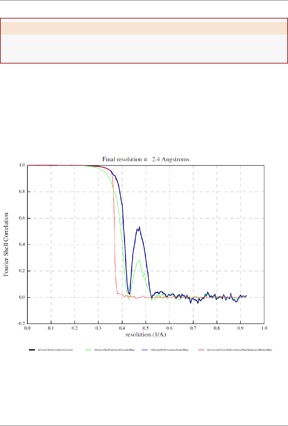
RELION
. Warning
You should not edit your STAR files because your current defocus values are fitted against the initial, slightly
wrong pixel size. Also, you should not use “Manually set pixel size” in the Extraction job. It will make metadata
inconsistent and break Bayesian Polishing. Thus, this option was removed in RELION 3.1.
7.2.2 Cs and the error in the pixel size
Recall that the phase shift due to defocus is proportional to the square of the wave number (i.e. inverse resolution),
while that due to spherical aberration is proportional to the forth power of the wave number. At lower resolutions, the
defocus term dominates and errors in the pixel size (i.e. errors in the wave number) can be absorbed into the defocus
value fitted at the nominal pixel size. At higher resolution, however, the Cs term becomes significant. Since Cs is not
fitted but given at the correct pixel size, the error persists. As the two terms have the opposite sign, the errors sometimes
cancel out at certain resolution shells, leading to a strange bump in the FSC curve. See an example below contributed
from a user. Here the pixel size was off by about 6 % (truth: 0.51 Å/px, nominal: 0.54 Å/px).
Below is a theoretical consideration. Let’s consider a CTF at defocus 5000 Å, Cs 2.7 mm at 0.51 Å/px. This is shown
in orange. If one thought the pixel size is 0.54 Å/px, the calculated CTF (blue) became quite off even at 5 Å (0.2).
7.2. Pixel size issues 121
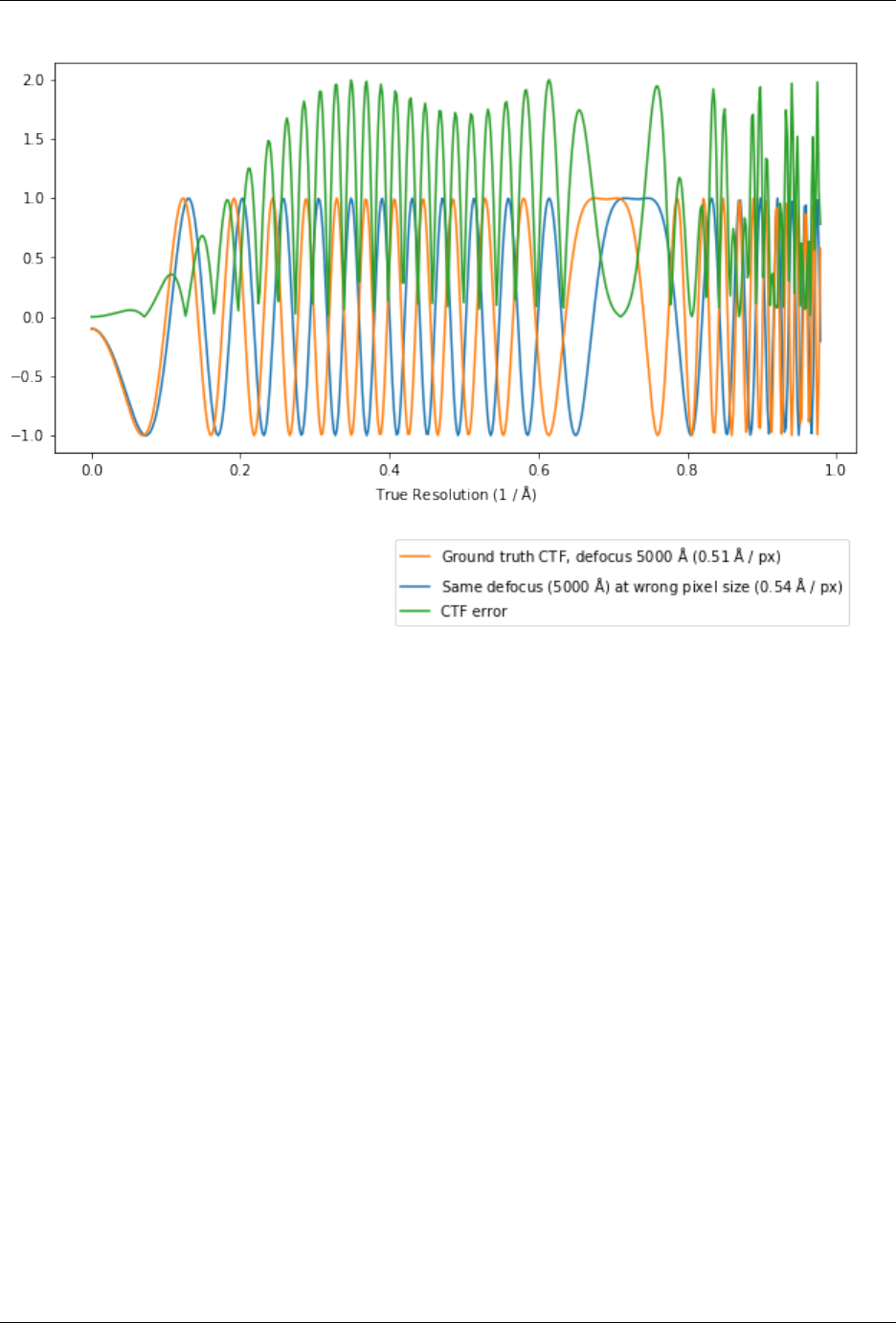
RELION
However, the defocus is fitted (by CtfFind, followed by CtfRefine) at 0.54 Å/px, the nominal pixel size. The defocus
became 5526 Å, absorbing the error in the pixel size. This is shown in blue. The fit is almost perfect up to about 3.3
Å. In this region, you can update the pixel size in PostProcess. Beyond this point, the error from the Cs term starts to
appear and the two curves go out of phase. This is why the FSC drops to zero. However, the two curves came into
phase again at about 1.8 Å (0.55)! This is why the FSC goes up again.
122 Chapter 7. Reference pages
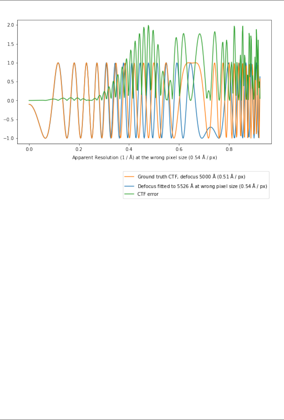
RELION
If you refine Cs and defocus simultaneously, the error in the pixel size is completely absorbed and the fit becomes
perfect. Notice that the refined Cs is 3.39, which is 2.7 * (0.54 / 0.51)^4. Also note that the refined defocus 5606 Å is
5000 * (0.54 / 0.51)^2.
7.2. Pixel size issues 123
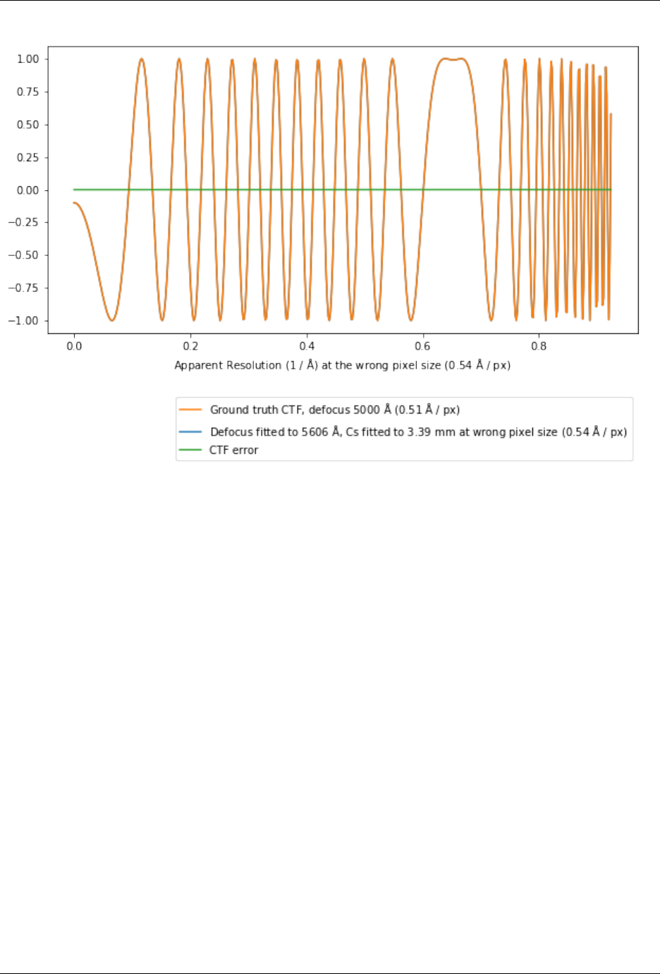
RELION
In practice, one just needs to run CtfRefine twice: first with Estimate 4th order aberrations to refine Cs,
followed by another run for defocus. Note that rlnSphericalAberration remains the same. The error in Cs is
expressed in rlnEvenZernike. You should never edit the pixel size in the STAR file!
Now everything is consistent at the nominal pixel size of 0.54 Å/px. In PostProcess, one should specify 0.51 Å/px to
re-scale the resolution and the header of the output map.
7.2.3 How can I merge datasets with different pixel sizes?
First of all: it is very common that one of your datasets is significantly better (i.e. thinner ice) than the others and merging
many datasets does not improve resolution. First process datasets individually and then merge the most promising two.
If it improves the resolution, merge the third dataset. Combining millions of bad particles simply because you have
them is a very bad idea and waste of storage and computational time!
For RELION 3.0, please see an excellent explanation posted to CCPEM by Max Wilkinson.
From RELION 3.1, you can refine particles with different pixel sizes and/or box sizes. Suppose you want to bring
polished (shiny) particles from the dataset2 project into the dataset1 project.
First, go to the Polish directory within the dataset1 project. Make a symbolic link to dataset2’s Polish/jobXXX by a
full path. A link by a relative path sometimes causes unexpected problems in RELION when it tries to expand paths.
If you are unlucky and the job number jobXXX is already present in the Polish directory of the dataset1 project, you
have to make a link by another name. In this case, you have to replace the file names in dataset2’s shiny.star.
Next, make sure they have different rlnOpticsGroupName. For example:
dataset1’s shiny.star:
124 Chapter 7. Reference pages

RELION
data_optics
loop_
_rlnOpticsGroup #1
_rlnOpticsGroupName #2
_rlnAmplitudeContrast #3
_rlnSphericalAberration #4
_rlnVoltage #5
_rlnImagePixelSize #6
_rlnMicrographOriginalPixelSize #7
_rlnImageSize #8
_rlnImageDimensionality #9
1 dataset1 0.100000 2.700000 300.000000 1.000000 1.000000␣
˓→ 140 2
dataset2’s shiny.star:
data_optics
loop_
_rlnOpticsGroup #1
_rlnOpticsGroupName #2
_rlnAmplitudeContrast #3
_rlnSphericalAberration #4
_rlnVoltage #5
_rlnImagePixelSize #6
_rlnMicrographOriginalPixelSize #7
_rlnImageSize #8
_rlnImageDimensionality #9
1 dataset2 0.100000 2.700000 300.000000 1.100000 1.100000␣
˓→ 128 2
Then use JoinStar. You don’t have to import; just go above the .Nodes directory to see the file from dataset2.
The result should look like:
data_optics
loop_
_rlnOpticsGroup #1
_rlnOpticsGroupName #2
_rlnAmplitudeContrast #3
_rlnSphericalAberration #4
_rlnVoltage #5
_rlnImagePixelSize #6
_rlnMicrographOriginalPixelSize #7
_rlnImageSize #8
_rlnImageDimensionality #9
1 dataset1 0.100000 2.700000 300.000000 1.000000 1.000000␣
˓→ 140 2
2 dataset2 0.100000 2.700000 300.000000 1.100000 1.100000␣
˓→ 128 2
Note that the dataset2’s rlnOpticsGroup has been re-numbered to 2.
7.2. Pixel size issues 125

RELION
If two datasets came from different detectors and/or had very different pixel sizes, you might want to apply MTF
correction during refinement. To do this, add two more columns: rlnMtfFileName to specify the MTF STAR file (the
path is relative to the project directory) and rlnMicrographOriginalPixelSize to specify the detector pixel size
(i.e. before down-sampling during extraction).
Refine this combined dataset. For a reference and mask, you must use the pixel size and box size of the first optics group
(or use --trust_ref_size option). The output pixel size and the box size will be the same as the input reference
map. After refinement, run CtfRefine with Estimate anisotropic magnification: Yes. This will refine the
relative pixel size difference between two datasets. In the above example, the nominal difference is 10 %, but it might
be actually 9.4 %, for example. Then run Refine3D again. The absolute pixel size of the output can drift a bit. It needs
to be calibrated against atomic models.
You can do similar things for other job types as long as you make all relevant paths consistent. For example, to run
Polish in a new project directory, you have to make sure the paths to raw movies, the gain reference and the motion
correction job are valid as well as paths to the particles and the references. For Polishing, do NOT merge MotionCorr
STAR files. First, run Polishing on one of the MotionCorr STAR files with run_data.star that contains all particles.
This will process and write only particles from micrographs present in the given MotionCorr STAR file. Repeat this for
the other MotionCorr STAR files. Finally, join two shiny.star files from the two jobs. The --only_group option
is not the right way to do Polishing on combined datasets.
7.2.4 How can I estimate the absolute pixel size of a map?
Experimentally and ideally, one can use diffraction from calibration standards.
Computationally, one can compare the map and a refined atomic model. However, if the model has been refined against
the same map, the model might have been biased towards the map. Also note that bond and angle RMSDs are not always
reliable when restraints are too strong.
If you are sure that 𝐶𝑠
true
given by the microscope manufacturer is accurate, which is often the case, AND the acceler-
ation voltage is also accurate, you can optimize the pixel size such that the apparent Cs fitted at the pixel size becomes
𝐶𝑠
true
.
First, find out the 𝑍
0
4
coefficient. This is the 7th number in rlnEvenZernike. The contribution of the spherical
aberration to the argument of the CTF’s sine function is 1/2𝜋𝜆
3
𝑘
4
𝐶𝑠, where k is the wave-number and 𝜆 is the
relativistic wavelength of the electron (0.0196 Å for 300 kV and 0.0251 Å for 200 kV). 𝑍
0
4
= 6𝑘
4
− 6𝑘
2
+ 1. By
comparing the 𝑘
4
term, we find the correction to the Cs is 12𝑍
0
4
/(𝜋𝜆
3
). Note that −6𝑘
2
+ 1 terms are cancelled by
the lower-order Zernike coefficients and can be ignored. Thus,
𝐶𝑠
apparent
= 𝐶𝑠
nominal
+ 12𝑍
0
4
* 10
−7
/(𝜋𝜆
3
).
10
−7
is to convert Cs from Å to mm. 𝐶𝑠
nominal
is what you used in CTFFIND (e.g. 2.7 mm for Titan and Talos).
The real pixel size can be calculated as NominalPixelSize(𝐶𝑠
true
/𝐶𝑠
apparent
)
1/4
.
7.2.5 Examples
In RELION 3.1, relion_refine (Refine3D, Class3D, MultiBody) stretches, shrinks, pads and/or crops input particles
so that the output has the same nominal pixel size and the box size as the input reference. Let’s study what happens in
various cases.
126 Chapter 7. Reference pages

RELION
One optics group
Suppose your optics group says 1.00 Å/px. If the header of your reference also says 1.00 Å/px, particles are used
without any stretching or shrinking. The output remains 1.00 Å/px.
Let’s assume that the nominal pixel size of 1.00 Å/px turns out slightly off and the real pixel size is 0.98 Å/px. As
discussed above, you should never change the pixel size in the optics group table, since all CTF parameters, coor-
dinates and trajectories are consistent with the nominal pixel size of 1.00 Å/px. When the header of your reference is
1.00 Å/px, the output map header says 1.00 Å/px, but it is actually 0.98 Å/px. Thus, you should specify 0.98 Å/px in
PostProcess. The post-processed map will have 0.98 Å/px in the header and the X-axis of the FSC curve will be also
consistent with 0.98 Å/px.
You must not use this 0.98 Å/px map from PostProcess in future Refine3D/MultiBody/Class3D jobs. Otherwise,
relion_refine stretches nominal 1.00 Å/px particles into 0.98 Å/px. Thus, the output map will have the nominal
pixel size of 0.98 Å/px but the actual pixel size will be 0.98 * 0.98 / 1.00 = 0.96 Å/px!
Multiple optics groups
Suppose your have two optics groups, one at 1.00 Å/px and the other at 0.95 Å/px. If the header of your reference is
1.00 Å/px, the particles in the first group are used without any stretching or shrinking, while those from the second
group are shrunk to match 1.00 Å/px. The output map is at 1.00 Å/px.
Let’s assume that the real pixel size of the first group is exactly at 1.00 Å/px, while that of the second group is actually
0.90 Å/px. After stretching by the ratio between the nominal pixel size and the pixel size in the reference header, the
true pixel size for the second group corresponds to 0.90 / 0.95 * 1.00 = 0.947 Å/px. Thus, the reconstruction is a
mixture of particles at 1.00 Å/px and 0.947 Å/px. Depending on the number and signal-to-noise ratio of particles in
each group, the real pixel size of the output can be any value between 0.947 and 1.00 Å/px, while the output header
says 1.00 Å/px.
Anisotropic magnification refinement in CtfRefine finds the relative pixel size differences between particles and the
reference. Suppose the actual pixel size of the output from Refine3D is 0.99 Å/px and there is no anistropic magni-
fication. CtfRefine finds the particles in the first group look smaller in real space than expected and puts 0.9900 0
0 0.9900 in rlnMatrix00, 01, 10, 11 (0.9900 = 0.99 / (1.00 * 1.00 / 1.00)). The particles in the second group
look larger in real space than expected and rlnMatrix00 to rlnMatrix11 will be 1.045 0 0 1.045 (= 0.99 / (0.90
/ 0.95 * 1.00)).
Notice that these numbers do not give you the absolute pixel size (e.g. 0.95 / 1.045 = 0.9091 ̸= 0.900). However,
you can work out the pixel size of the reconstruction and other optics groups if you are confident with the pixel size
of one optics group. You can also work out the pixel size of all optics groups if you calibrate the pixel size of the
reconstruction with atomic models. Carefully follows two streching/shrinking steps done in relion_refine: one to
match the nominal pixel size of an optics group to the nominal pixel size of the reference and the further correction by
rlnMatrix.
7.3 Automation: Schemes
Schemes were introduced to relion-3.1, where they were called Schedules but to prevent confusion with scheduled jobs
in the main GUI, they were renamed to Schemes in relion-4.0 and their functionality was further improved. Schemes aim
to provide a generalised methodology for automatic submission of relion jobs. This is useful for creating standardised
workflows, for example to be used in on-the-fly processing. The relion_it.py script that was introduced in relion-3.1
has been re-written to work with the Schemes.
The Schemes framework is built around the following key concepts: a directed graph that represents the logic of a series
of subsequent relion job-types is encoded in Nodes and Edges. Nodes can be either a relion job or a so-called Operator;
Edges form the connections between Nodes. In addition, Schemes have their own Variables.
7.3. Automation: Schemes 127

RELION
All information for each Scheme is stored in its own subdirectory of the Schemes/ directory in a relion project, e.g.
Schemes/prep. Within each Scheme’s directory, the scheme.star file contains information about all the Variables,
Edges, Operators and Jobs.
7.3.1 Variables
Three different types of Variables exist: floatVariables are numbers; booleanVariables are either True or False; and
stringVariables are text. Each Variable has a VariableName; a so-called VariableResetValue, at which the value is
initialised; and a VariableValue, which may change during execution of the Scheme through the actions of Operators,
as outlined below.
One special stringVariable is called email. When this is set, upon completion or upon encountering an error, the
Scheme will send an email (through the Linux mail command) to the value of the email stringVariable.
7.3.2 Jobs
Jobs are the first type of Node. They can be of any of the jobtypes defined in the relion pipeliner, i.e. Import
,
Motion correction , etc, including the new External . Any Variable defined in the Scheme can be set as a parameter
in a Job, by using two dollar signs on the GUI or in the job.star file. For example, one could define a floatVariable
voltage and use $$voltage on the corresponding input line of an Import job. Upon execution of the job inside the
Scheme, the $$voltage will be replaced with the current value of the voltage floatVariable.
Jobs within a Scheme each have a JobName and a JobNameOriginal. The latter is defined upon creation of the job (see
next section); the former depends on the execution status of the Scheme, and will be set to the executed relion job’s
name, e.g. CtfFind/job004. In addition, each job has a JobMod and a jobHasStarted status. There are two types of
JobMode:
new
regardless of jobHasStarted, a new job will be created, with its own new JobName, every time the Schemer
passes through this Node.
continue
if jobHasStarted is False, a new job, with its own new JobName, will be created. If jobHasStarted is True, the
job will be executed as a continue job inside the existing JobName directory.
When a Scheme executes a Job, it always sets jobHasStarted to True. When a Scheme is reset, the jobHasStarted status
for all jobs is set to False.
7.3.3 Operators
Operators are the second type of Node. Each operator within a Scheme has a unique name and a type. Operators can
also have an output Variable: output, on which they act, and up to two input Variables: input1 and input2. Most, but
not all operators change the value of their output Variable.
The following types of operators act on an output that is a floatVariable:
float=set
output = floatVariable input1
float=plus
output = floatVariable input1 + floatVariable input2
float=minus
output = floatVariable input1 - floatVariable input2
128 Chapter 7. Reference pages

RELION
float=mult
output = floatVariable input1 × floatVariable input2
float=divide
output = floatVariable input1 / floatVariable input2
float=round
output = ROUND(floatVariable input1)
float=count_images
sets output to the number of images in the STAR file with the filename in stringVariable input1. stringVariable
input2 can be particles, micrographs or movies, depending on what type of images need to be counted.
float=count_words
sets output to the number of words in stringVariable input1, where individual words need to be separated with a
, (comma) sign.
float=read_star
sets output to the value of a double or integer that is read from a STAR file. stringVariable input1 defines
which variable to read as: starfilename,tablename,metadatalabel. If tablename is a table instead of a list, then
floatVariable input2 defines the line number, with the default of zero being the first line.
float=star_table_max
sets output to the maximum value of a column in a starfile table, where stringVariable input1 specifies the column
as starfilename,tablename,metadatalabel.
float=star_table_min
sets output to the minimum value of a column in a starfile table, where stringVariable input1 specifies the column
as starfilename,tablename,metadatalabel.
float=star_table_avg
sets output to the average value of a column in a starfile table, where stringVariable input1 specifies the column
as starfilename,tablename,metadatalabel.
float=star_table_sort_idx
a sorting will be performed on the values of a column in a starfile table, where stringVariable input1 specifies the
column as starfilename,tablename,metadatalabel. stringVariable input2 specifies the index in the ordered array:
the lowest number is 1, the second lowest is 2, the highest is -1 and the one-but-highest is -2. Then, output is set
to the corresponding index in the original table.
The following types of operators act on an output that is a booleanVariable:
bool=set
output = booleanVariable input1
bool=and
output = booleanVariable input1 AND booleanVariable input2
bool=or
output = booleanVariable input1 OR booleanVariable input2
bool=not
output = NOT booleanVariable input1
bool=gt
output = floatVariable input1 > floatVariable input2
bool=lt
output = floatVariable input1 < floatVariable input2
bool=ge
output = floatVariable input1 >= floatVariable input2
7.3. Automation: Schemes 129

RELION
bool=le
output = floatVariable input1 <= floatVariable input2
bool=eq
output = floatVariable input1 == floatVariable input2
bool=file_exists
output = True if a file with the filename stored in stringVariable input1 exists on the file system; False otherwise
bool=read_star
reads output from a boolean that is stored inside a STAR file. stringVariable input1 defines which variable to
read as: starfilename,tablename,metadatalabel. If tablename is a table instead of a list, then floatVariable input2
defines the line number, with the default of zero being the first line.
The following types of operators act on an output that is a stringVariable:
string=set
output = stringVariable input1
string=join
output = concatenate stringVariable input1 and stringVariable input2
string=before_first
sets output to the substring of stringVariable input1 that occurs before the first instance of substring stringVari-
able input2.
string=after_first
sets output to the substring of stringVariable input1 that occurs after the first instance of substring stringVariable
input2.
string=before_last
sets output to the substring of stringVariable input1 that occurs before the last instance of substring stringVariable
input2.
string=after_last
sets output to the substring of stringVariable input1 that occurs after the last instance of substring stringVariable
input2.
string=read_star
reads output from a string that is stored inside a STAR file. stringVariable input1 defines which variable to read
as: starfilename,tablename,metadatalabel. If tablename is a table instead of a list, then floatVariable input2
defines the line number, with the default of zero being the first line.
string=glob
output = GLOB(stringVariable input1), where input1 contains a Linux wildcard and GLOB is the Linux function
that returns all the files that exist for that wildcard. Each existing file will be separated by a comma in the output
string.
string=nth_word
output = the Nth substring in stringVariable input1, where N=*floatVariable* input2, and substrings are separated
by commas. Counting starts at one, and negative values for input2 mean counting from the end, e.g. input2=-2
means the second-last word.
The following types of operators do not act on any variable:
touch_file
performs touch input1 on the file system
copy_file
performs cp input1 input2 on the file system. stringVariable input1 may contain a linux wildcard. If string-
Variable input2 contains a directory structure that does not exist yet, it will be created.
130 Chapter 7. Reference pages

RELION
move_file
performs mv input1 input2 on the file system. stringVariable input1 may contain a linux wildcard. If string-
Variable input2 contains a directory structure that does not exist yet, it will be created.
delete_file
performs rm -f input1 on the file system. stringVariable input1 may contain a linux wildcard.
email
sends an email, provided a stringVariable with the name email exists and the Linux command mail is functional.
The content of the email has the current value of stringVariable input1, and optionally also stringVariable input2.
wait
waits floatVariable input1 seconds since the last time this operator was executed. The first time it is executed,
this operator only starts the counter and does not wait. Optionally, if output is defined as a floatVariable, then
the elapsed number of seconds since last time is stored in output.
exit_maxtime
terminates the execution of the Scheme after the number of hours have passed since its start as stored in float-
Variable input1.
exit
terminates the execution of the Scheme.
7.3.4 Edges
Two types of Edges exist. The first type is a normal Edge, which connects an inputNode to an ouputNode, thereby
defining their consecutive execution.
The second type is called a Fork. A Fork has one inputNode, an outputNode, an outputNodeIfTrue, and an associated
booleanVariable. Whether one or the other output Node is executed depends on the current value of the booleanVariable
that is associated with the Fork. The fork with lead from the inputNode, an outputNode if the booleanVariable is False.
The fork will lead from the inputNode, an outputNodeIfTrue if the booleanVariable is True. Thereby, Forks are the
main instrument of making decisions in Schemes.
7.3.5 Create a Scheme
The combination of the Variables, Nodes and Edges allows one to create complicated sequences of jobs. It is probably
a good idea to draw out a logical flow-chart of your sequence before creating a Scheme. Then, use your favourite
text editor to manually edit the files Schemes/SCHEMENAME/scheme.star and all the files Schemes/SCHEMENAME/
JOBNAMES/job.star for all the jobs in that Scheme. Following the prep and proc examples in the scripts directory
of your relion installation is probably the easiest way to get started.
In the Schemes/SCHEMENAME/scheme.star file, first add all the different variables and operators that you will need.
Note that any variable names that contain a JobNameOriginal of any of the Jobs inside any Scheme that is present
in the ProjectDirectory, will be replaced by the current JobName upon execution of an operator. For example, a
stringVariable with the value Schemes/prep/ctffind/micrographs_ctf.star will be replaced to something like
CtfFind/job003/micrographs_ctf.star upon execution of the job that uses it, assuming that the current JobName
of that job is CtfFind/job003/ in the Schemes/prep/scheme.star file.
Then, add your jobs. You can use the normal relion GUI to fill in all parameters of each job that you need and then use the
Save job.star options from the Jobs menu to save the job.star file in the corresponding Schemes/SCHEMENAME/
JOBNAMES/ directory. Jobs use the same mechanism as described for the Variables above. So, if an Auto-picking job
depends on its micrographs STAR file input on a CTF estimation job called ctffind, and this CTF estimation job is part of
a Scheme called prep, then the micrographs STAR file input for the Auto-picking job should be set to Schemes/prep/
ctffind/micrographs_ctf.star, and this will be converted to CtfFind/job003/micrographs_ctf.star upon
7.3. Automation: Schemes 131
RELION
execution of the job. In addition, a corresponding edge will be added to the default_pipeliner.star upon execution
of the Scheme. Also note that parameters in job.star files may be updated with the current values of Variables from
the Scheme by using the $$ prefix, followed by the name of the corresponding Variable, as also mentioned above.
In addition, the JobMode needs to be chosen from options: new or continue. Typically, in on-the-fly-processing
procedures that iterate over ever more movies, jobs like Import , Motion correction , CTF estimation , Auto-picking
and Particle extraction are set as continue, whereas most other jobs are set as new.
Finally, once all the Variables, Operators and Jobs are in place, one should define all the Edges between them.
The Scheme will be initialised (and reset) to the left-hand Node of the first defined Edge. If the Scheme is not an infinite
loop, it is recommended to add the exit Operator as the last Node.
Once a Scheme has been created, it may be useful for more than one relion project. Therefore, you may want to store
it in a tar-ball:
tar -zcvf preprocess_scheme.tar.gz Schemes/preprocess
That tar-ball can then be extracted in any new relion project directory:
tar -zxvf preprocess_scheme.tar.gz
Executing a Scheme
Once you have created the Scheme/name/ (sub)directories (with “name” being the name of your scheme), you can
launch a separate GUI using:
relion_schemegui.py name
You can start, stop, change parameters, and restart the scheme from there. You can also look into this python script to
see the actual calls it makes to relion_schemer, which is the command line program that executes the scheme. While it
runs, you can then follow the generation of new jobs in the normal relion GUI.
7.4 Helical reconstruction
Shaoda He, a PhD-student in the Scheres group, implemented a workflow for the processing of helical assem-
blies. This involves additional tabs to the parameter-panels of the Auto-picking , Particle extraction , 2D classification ,
3D classification , 3D auto-refine , Particle polishing and Mask create job-types. We do not have a separate tutorial for
processing helical assemblies. The general principles remain the same as for single-particle analysis, which is covered
in this tutorial. Therefore, users intending to use relion for helical processing are still encouraged to do this tutorial
first. For a detailed description of the helical options, the user is referred to the corresponding pages on the RELION
wiki, or to Shaoda’s paper[HS17]. We are aware that a tutorial on helical processing is probably overdue, but due to
time constraints we haven’t got to doing that yet. Sorry. ..
132 Chapter 7. Reference pages

RELION
7.4.1 Initial model generation for amyloids
The relion_helix_inimodel2d program is a new feature in relion-3.1. It allows generation of an initial 3D reference
for helical reconstruction, in particular for amyloids. It is run from the command line, and takes a selection of suitable
2D class averages as input. It will try to align these class averages with respect to each other to form a continuously
changing density that spans an entire cross-over. At the heart of the iterative refinement process lies a tomographic 2D
reconstruction with all 1D pixel columns from the cross-over. Details of this program, together with a more elaborate
documentation of its functionality remain to be published. Possible usage is:
relion_helix_inimodel2d --i Select/job056/class_averages.star \
--crossover_distance 800 --angpix 1.15 --maxres 9 --search_shift 3 \
--mask_diameter 250 --j 6 --iter 5 --o IniModel/run1
relion_helix_inimodel2d --i IniModel/run1_it005.star \
--iniref 1@IniModel/run1_it005_reconstructed.mrcs --angpix 1.15 \
--maxres 6 --search_angle 2 --step_angle 0.5 --mask_diameter 250 \
--j 6 --iter 5 --o IniModel/run2
We like xmipp-2.4 for live-updated display of the following images during the optimisation:
xmipp_show -img rec.spi after_reproject.spi before_reproject.spi -poll &
7.5 Subtomogram Averaging
7.5.1 Data Types
The custom data types used in tomography programs in relion are:
Tomogram set
The tomogram set describes all the tomograms (i.e. tilt series) defined in a project, and is usually named tomograms.
star. It contains a single table, named global, which defines the properties pertaining to each tomogram. Each row
corresponds to one tomogram, and it lists the following properties:
• The tomogram name (rlnTomoName): a unique identifier used to refer to this tomogram within the entire project
(i.e. within the tomogram set, the particle set and the trajectory set)
• The tilt series file name (rlnTomoTiltSeriesStarFile): the path to the star file corresponding to each to-
mogram/image stack
• The tomogram size (rlnTomoSize<X/Y/Z>): the extent of the tomogram region in 3D space
• The handedness (rlnTomoHand): this value is either +1 or -1, and it describes whether the focus increases or
decreases as a function of depth (projected Z coordinate). It cannot be known a priori and has to be determined
experimentally. It is typically identical across the entire data set.
• The pixel size of the raw micrographs, given in Å (rlnMicrographOriginalPixelSize)
• The pixel size of the tilt series, given in Å (rlnTomoTiltSeriesPixelSize), corresponding to the dimensions
given by rlnTomoSize<X/Y/Z>, after the binning applied in the Motion correction job
• The tomogram binning (rlnTomoTomogramBinning): the binning applied to the tilt series in
rlnTomoTiltSeriesStarFile to reconstruct the tomogram in rlnTomoReconstructedTomogram
7.5. Subtomogram Averaging 133

RELION
• The reconstructed tomogram file (rlnTomoReconstructedTomogram): the path to the reconstructed tomo-
gram mrc file, at the binning in rlnTomoTomogramBinning
• The Etomo file (rlnEtomoDirectiveFile)
• The optics group name (rlnOpticsGroupName)
• The voltage, given in kV (rlnVoltage)
• The spherical aberration, given in mm^-1 (rlnSphericalAberration)
• The amplitude contrast (rlnAmplitudeContrast)
The star file for each tomogram, to which rlnTomoTiltSeriesStarFile points, contains a single table with the
same name as the tomogram. In it, each row corresponds to one tilt image and includes the following properties,
among others:
• The tilt image rotation angles and shifts (rlnTomo<X/Y>Tilt, rlnTomoZRot and rlnTomo<X/
Y>ShiftAngst)
• The astigmatic defocus (rlnDefocus<U/V> and rlnDefocusAngle)
• The intensity scale factor related to effective ice thickness at each tilt angle (rlnCtfScalefactor)
• The cumulative radiation dose (rlnMicrographPreExposure)
• The frame count (rlnTomoTiltMovieFrameCount)
Particle set
The particle set (typically named particles.star) lists all the particles in a data set. It is roughly equivalent to
the corresponding particles file used by the SPA programs in relion, and it serves as the binding element between the
tomography programs and the ones used for the general refinement.
Like an SPA particle set, the tomography particle set consists of an optics table and a particles table. Unlike in
an SPA particle set, the coordinates of the particles are given in 3 dimensions (rlnCenteredCoordinate<X/Y/
Z>Angst and rlnOrigin<X/Y/Z>Angst), and each particle also requires a tomogram name (rlnTomoName) that
identifies the particle’s tomogram of origin, as defined in the tomogram set. Note that in Relion 5, the pixel coordinates
rlnCoordinate<X/Y/Z> have been replaced by the absolute and centered coordinates rlnCenteredCoordinate<X/
Y/Z>Angst, which are in Angstroms from the centre of the tomogram.
Also unlike in SPA, the tomography particles should not be thought of as pixel data stored on disk, but instead as
abstract entities defined in this file. They are represented on the disk either as 2D stacks of CTF-premultiplied ex-
tracted images (the preferred way in Relion 5) or as 3D volumes where Fourier slices of the 2D images are combined
in 3D. The particles that are used for refinement (i.e. the pseudo-subtomograms) can be created using the program
relion_tomo_subtomo, but they should be regarded as transient data that become invalid once any of the other prop-
erties of their tomograms have been updated. Therefore, during the processing of a tomography data set, the pseudo-
subtomograms are typically created multiple times.
Another difference to a SPA 2D particle set is that tomography particles can optionally possess two different ori-
entations. In tomography, the approximate orientation of a particle is often dictated by the geometric context (e.g.
the orientation of a membrane in which they are embedded). Therefore, the subtomogram alignment can be greatly
accelerated by defining the initial orientation of each subtomogram in relation to that geometry (using the fields
rlnTomoSubtomogram<Rot/Tilt/Psi>) and then applying strong priors during refinement to constrain the angles
that describe the orientation of the particle itself with respect to its subtomogram (rlnAngle<Rot/Tilt/Psi>). Since
only the latter angles are considered by relion_refine, the priors will only affect those angles. Typically, this means
that the rlnAngleTilt angle will be constrained, while the other two are usually unknown, even in tomography.
134 Chapter 7. Reference pages

RELION
Trajectory set
The trajectory set (typically named motion.star) contains the motion trajectories of all particles in a corresponding
particle set. The trajectories can be estimated using the program relion_tomo_align, and they will be considered by
any relion tomography program that requires particle positions.
The trajectory file consists of P+1 tables, where P is the number of particles in the corresponding particle set. The first
table only contains the number of particles, while every successive table, named using the particle name (the same as
the value of rlnTomoParticleName in the particle set file) lists the trajectory of each particle. The trajectories are
given in Å, and they are relative to the position of the particle in the chronologically first tilt image (i.e. the image with
the lowest cumulative dose).
Optimisation set
The optimisation set is the central data type in a relion tomography project, and it only contains paths to other files. It
is usually named optimisation_set.star.
Specifically, it can point to the following data files:
• A tomogram set listing all tomograms.
• A particle set listing all particles.
• A trajectory set describing the motion of all particles.
All of those entries are optional, and different programs require different inputs. All programs take an optimisation
set as input, and most of them also write one out. If a data file is created or updated by a program, it is added to the
optimisation set that the program writes out. This frees the user from having to track which programs update which
data files. For example, relion_tomo_refine_ctf will only update the tomogram set, because the defoci are only defined
once for each tilt image, while relion_tomo_align will update the tomogram set, the particle set and the trajectory set.
When running a program, the individual data files can also be specified separately, in which case the individual files will
override the ones listed in the optimisation set. This allows the user to easily perform the same procedure with specific
data files exchanged. If all data files required by a program have been specified individually, then an optimisation set
is not required at all.
There are 3 ways to create an initial optimisation set:
• Use the utility program relion_tomo_make_optimisation_set.
• Run any program and specify the individual data files. The program will then output a new optimisation set.
• Write one manually.
7.5.2 Programs
These are the most relevant tomography-related programs in relion:
7.5. Subtomogram Averaging 135

RELION
relion_tomo_reconstruct_particle
This program constructs high-resolution 3D reference maps from a given optimisation set. It is similar to
relion_reconstruct, except that it does not require pre-extracted particle images. Instead, it extracts square win-
dows of arbitrary size (--b argument) directly from the tilt series and it uses those for the reconstruction (using Fourier
inversion). It considers the defoci of the individual particles, as well as particle motion and higher-order aberrations.
The output consists of a pair of maps (one for each half set) as well as a merged map. In addition, the numerator (data
term) and denominator (weight term) (see Eq. 3 in the |RELION| paper) of all 3 maps are also written out to facilitate
further processing.
Relevant program arguments:
• --i and/or --p, --t and --mot: input optimisation-set and/or its components (see optimisation set).
• --b: box size of the reconstruction. Note that this is independent of the box size used to refine the particle.
This allows the user to construct a 3D map of arbitrary size to gain an overview of the structure surrounding the
particle. A sufficiently large box size also allows more of the high-frequency signal to be captured that has been
delocalised by the CTF.
• --crop: cropped box size. If set, the program will output an additional set of maps that have been cropped to this
size. This is useful if a map is desired that is smaller than the box size required to retrieve the CTF-delocalised
signal.
• --bin: downsampling (binning) factor. Note that this does not alter the box size. The reconstructed region
instead becomes larger.
• --SNR: apply a Wiener filter with this signal-to-noise ratio. If omitted, the reconstruction will use a heuristic to
prevent divisions by excessively small numbers. Please note that using a low (even though realistic) SNR might
wash out the higher frequencies, which could make the map unsuitable to be used for further refinement.
• --sym: name of the symmetry class (e.g. C6 for six-fold point symmetry).
• --mem: (approximate) maximum amount of memory to be used for the reconstruction (see below).
• --j: number of threads used for the non-reconstruction parts of the program (e.g. symmetry application or
gridding correction). This should be set to the number of CPU cores available.
• --j_out: number of threads that compute partial reconstructions in parallel. This is faster, but it requires
additional memory for each thread. When used together with the --mem argument, this number will be reduced
to (approximately) maintain the imposed memory limitation.
• --j_in: number of threads to be used for each partial reconstruction. This is a slower way to parallelise the
procedure, but it does not require additional memory. Unless memory is limited, the --j_out option should be
preferred. The product of --j_out and --j_in should not exceed the number of CPU cores available.
• --o: name of the output directory (that will be created).
136 Chapter 7. Reference pages

RELION
Program output:
After running the program, the output directory (--o argument) will contain the following items:
• <half1/half2/merged>.mrc: the reconstructed cropped maps.
• <half1/half2/merged>_full.mrc: the reconstructed full-size maps, in case the full size (--b argument) differs
from the cropped size (--crop argument).
• data_<half1/half2/merged>.mrc: the reconstructed data term at full size.
• weight_<half1/half2/merged>.mrc: the reconstructed weight term at full size.
• note.txt: a text file containing the command issued to run the program.
relion_tomo_subtomo
This program creates pseudo subtomograms that can be fed into relion_refine to perform subtomogram alignment.
Those pseudo subtomograms are not meant to represent the actual density distributions of the particles, but instead
abstract 3D image terms that allow relion_refine to approximate the cost function that would arise if the alignment
were to be performed on the stack of corresponding 2D images instead. Specifically, each pseudo subtomogram consists
of a sum of CTF-weighted observations (data term) as well as the corresponding sum of CTF
2
terms (weight term). In
addition, the output weight term also contains - concatenated along the Z axis - a 3D multiplicity-image (number of
Fourier slices contributing to each Fourier voxel) that allows relion_refine to estimate a spherically symmetrical
noise distribution.
The reconstructed pseudo subtomograms consider the motion of the particles as well as higher-order aberrations, if
either have been estimated. The program will output a new particle set, as well as a new optimisation set in which the
initial particle set has been replaced by the newly generated one. That particle set can be fed into relion_refine.
If a subtomogram orientation has been defined (see particle set), then the subtomogram will be constructed in that
coordinate system. If the approximate orientation of the particle is known a-priori from the surrounding geometry, this
allows angle priors to be used in relion_refine to avoid searching through implausible orientations. In particular, for
particles sampled from a manifold (using relion_tomo_sample_manifold), the Z axis of the subtomogram coordinate-
system is always perpendicular to the local manifold. A strong tilt-angle prior can then be applied to only search
through orientations that do not tilt the particle too far away from that orientation, while leaving the remaining two
angles unconstrained (i.e. the direction of tilt and the rotation around the Z axis).
Relevant program arguments:
• --i and/or --p, --t and --mot: input optimisation-set and/or its components (see optimisation set).
• --b: initial box size of the reconstruction. A sufficiently large box size allows more of the high-frequency signal
to be captured that has been delocalised by the CTF.
• --crop: cropped output box size. After construction, the resulting pseudo subtomograms are cropped to this
size. A smaller box size allows the (generally expensive) refinement using relion_refine to proceed more
rapidly.
• --bin: downsampling (binning) factor. Note that this does not alter the initial or the cropped box size. The
reconstructed region instead becomes larger.
• --cone_weight: downweight a cone in Fourier space along the Z axis (as defined by the coordinate system of
the particle). This is useful for particles embedded in a membrane, as it can prevent the alignment from being
driven by the membrane signal (the signal of a planar membrane is localised within one line in 3D Fourier space).
Note that the coordinate system of a particle is given by both the subtomogram orientation (if defined) and the
7.5. Subtomogram Averaging 137

RELION
particle orientation (see particle set). This allows the user to first obtain a membrane-driven alignment, and to
then specifically suppress the signal in that direction.
• --cone_angle: the (full) opening angle of the cone to be suppressed, given in degrees. This angle should
include both the uncertainty about the membrane orientation and its variation across the region represented in
the subtomogram.
• --j: number of threads used to reconstruct pseudo subtomograms in parallel. Each thread will require additional
memory, so this should be set to the number of CPU cores available, unless the memory requirements become
prohibitive.
• --o: name of the output directory (that will be created).
Program output:
After running the program, the output directory (--o argument) will contain the following items:
• particles.star: a new particle set containing the file names of the reconstructed subtomograms. This file can be
understood by relion_refine
• optimisation_set.star: a new optimisation set pointing to the new particle set.
• Subtomograms/<**`particle_name`>_data.mrc**: 3D images representing the data terms of all subtomo-
grams.
• Subtomograms/< particle_name >_weights.mrc: the weight terms of all subtomograms. Each 3D image
contains, concatenated along Z, an image describing the sums over all CTF
2
and an image describing the multi-
plicities.
• note.txt: a text file containing the command issued to run the program.
relion_tomo_align
This program refines the projections that map 3D space onto the images of the tilt series, as well as (optionally) also
the beam-induced motion trajectories of the particles. Each projection is optimised using the full 5 degrees of freedom:
the assumption of a common tilt axis is abandoned. Even if no beam-induced motion is estimated, the (in that case
static) 3D particle-positions are also optimised by the program. This is because those 3D positions cannot be assumed
to be known in advance, since they have only been inferred from the observed 2D particle-positions in the individual
tilt images. Therefore, this program always looks for the optimal set of 3D positions and projections.
If the particle motion is also being estimated (using the --motion argument), then the 3D positions of the particles are
allowed to differ between tilt images, albeit only in a limited and spatially smooth manner. This is done analogously to
Bayesian polishing in 2D (implemented in relion_motion_refine), except that the trajectories are estimated in 3D,
and that no acceleration constraint is imposed. Because part of the particle motion is rigid, the motion estimation also
always includes a rigid alignment of the frames.
Please note that estimating beam-induced motion significantly increases the runtime of the program, so it should only
be done in the final rounds of optimisation.
The estimated particle trajectories are written into the output trajectory set, the projection matrices (containing the rigid
part of the motion as well as the alignment of the tilt series - these cannot be distinguished) into the output tomogram set
and the estimated (initial) particle positions into the output particle set which replace the given trajectory, tomogram
and particle sets in the output optimisation set.
138 Chapter 7. Reference pages

RELION
General program arguments:
• --i and/or --p, --t, --mot, --ref<1/2>, --mask and --fsc: input optimisation-set and/or its components
(see optimisation set).
• --b: box size to be used for the estimation. Note that this can be larger than the box size of the reference map.
A sufficiently large box size allows more of the high-frequency signal to be captured that has been delocalised
by the CTF.
• --r: maximal assumed error in the initial 2D particle-positions (distances between the projected 3D positions
and their true positions in the images), given in pixels.
• --j: number of threads to be used. This should be set to the number of CPU cores available.
• --o: name of the output directory (that will be created).
Motion-related arguments:
• --motion: perform motion estimation simultaneously with the tilt-image alignment.
• --s_vel: the expected amount of motion (i.e. the std. deviation of particle positions in Å after 1 electron per
Å
2
of radiation).
• --s_div: the expected spatial smoothness of the particle trajectories (a greater value means spatially smoother
motion).
• --sq_exp_ker: assume that the correlation of the velocities of two particles decays as a Gaussian over their
distance, instead of as an exponential. This will produce spatially smoother motion and result in a shorter program
runtime.
Deformation-related arguments:
• --deformation: perform 2D deformation estimation for each tilt-image.
• --def_w: Number of horizontal sampling points for the deformation grid.
• --def_h: Number of vertical sampling points for the deformation grid.
• --def_model: Type of model to estimate deformations (linear, spline or Fourier).
• --def_reg (0.0): Value of the deformation regulariser
• --per_frame_deformation: Model separate 2D deformations for each tilt-image instead of the whole tilt
series.
Program output:
After running the program, the output directory (--o argument) will contain the following items:
• motion.star: a new trajectory set
• tomograms.star: a new tomogram set containing the newly estimated projection matrices (rlnTomoProj<X/
Y/Z/W>)
• particles.star: a new particle set containing the newly estimated particle positions in 3D (rlnCoordinate<X/
Y/Z>)
• optimisation_set.star: a optimisation set pointing to the new trajectory, tomogram and particle sets.
7.5. Subtomogram Averaging 139

RELION
• Trajectories/< tomogram_name >_x<1/8>.ply: meshes of 3D trajectories in ply format, scaled by a fac-
tor of 1 or 8, respectively. Note that only the trajectories themselves are scaled - their positions are those
of the particles. They can be viewed in relation to (low-magnification) tomograms as produced by re-
lion_tomo_reconstruct_tomogram in a viewer that supports both meshes and 3D images (such as e.g. Paraview).
• note.txt: a text file containing the command issued to run the program.
relion_tomo_refine_ctf
This program estimates the astigmatic defoci of the individual tilt images, the ice thickness (which determines the
overall signal intensity) and higher-order optical aberrations.
Defocus: In tomography, the relative depth distances between particles are known from the 3D positions of the particles.
Therefore, only one defocus value is estimated for all the particles in each tilt image. Because of the often large number
of particles in each tomogram, this value can typically be estimated to greater precision than in single-particle analysis,
where the defocus of each particle has to be estimated independently.
Ice-thickness: A thicker sample permits fewer electrons to pass through, which reduces the scale of the signal. In
addition to the actual variation in sample thickness, the effective thickness of the ice also increases as the sample is
tilted. This program allows the user to estimate the signal intensity either independently for each tilt image, or by fitting
the base thickness, the initial beam luminance and the surface normal of the sample assuming Beer-Lambert’s Law.
In the latter case, only one surface normal and base thickness are estimated for an entire tilt series, which allows for a
more stable fit from tomograms with fewer particles.
Higher-order optical aberrations: This algorithm works analogously to relion_ctf_refine for single-particle
analysis. As in single-particle analysis, the aberrations are estimated per optics group. This allows the user to group
particles that are expected to share the same aberrations, either by image region or by subset of tilt series, or both. Both
symmetrical (even) and antisymmetrical (odd) aberrations are supported. A detailed description of the aberrations
estimation algorithm can be found in the relion aberrations paper.
The estimated defocus and ice-thickness values are written into the output tomogram set and the aberrations into the
particle set, both of which replace the given sets in the output optimisation set.
General program arguments:
• --i and/or --p, --t, --mot, --ref<1/2>, --mask and --fsc: input optimisation-set and/or its components
(see optimisation set).
• --b: box size to be used for the estimation. Note that this can be larger than the box size of the reference map.
A sufficiently large box size allows more of the high-frequency signal to be captured that has been delocalised
by the CTF.
• --j: number of threads to be used. This should be set to the number of CPU cores available.
• --o: name of the output directory (that will be created).
140 Chapter 7. Reference pages

RELION
Defocus-estimation arguments:
• --do_defocus: instructs the program to estimate the defoci.
• --do_reg_defocus: applies defocus regularisation. High-tilt images do not offer enough signal to recover the
defocus value precisely. The regularisation forces the estimated defoci to assume similar values within a given
tilt series, which prevents those high-tilt images from overfitting.
• --lambda: defocus regularisation strength.
• --d0 and --d1: minimal and maximal defocus offset (from the initial value) to scan in the initial part of the
defocus estimation. This scan allows the algorithm to escape a local minimum in case it has been intialised in
one. Afterwards, a local astigmatic-defocus refinement is performed. Both values are assumed to be given in Å.
• --ds: number of steps between --d0 and --d1.
• --kmin: Lowest spatial frequency to consider, in Å.
• --reset_to_common: Reset the CTFs of all tilts to a common one prior to local refinement.
Ice-thickness estimation arguments:
• --do_scale: instructs the program to estimate the signal scale or ice thickness.
• --per_frame_scale: estimate the signal-scale parameter independently for each tilt. If not specified, the ice
thickness, beam luminance and surface normal are estimated instead. Those three parameters then imply the
signal intensity for each frame. Due to the smaller number of parameters, the ice thickness model is more robust
to noise. By default, the ice thickness and surface normal will be estimated per tilt-series, and the beam luminance
globally.
• --per_tomogram_scale: estimate the beam luminance separately for each tilt series. This is not recommended.
Aberrations-estimation arguments:
• --do_even_aberrations: instructs the program to estimate the even (i.e. symmetrical) aberrations. These
deform the shape of the CTF.
• --do_odd_aberrations: instructs the program to estimate the odd (i.e. anti-symmetrical) aberrations. These
rotate the phases of the observed images.
• --ne: number of Zernike bands used to fit the even aberrations. A greater number can quickly lead to overfitting.
The user is advised to keep this value at 4 - this will allow for a correction to the spherical aberration term, as
well as four-fold and first- and second-order two-fold astigmatism.
• --no: number of odd Zernike bands. The user is advised to keep this value at 3 - this will allow for beam tilt
and three-fold astigmatism.
7.5. Subtomogram Averaging 141

RELION
Program output:
After running the program, the output directory (--o argument) will contain the following items:
• tomograms.star: a new tomogram set containing the newly estimated defoci (rlnDefocus<U/V> and
rlnDefocusAngle) and ice thickness values. Note that only the signal scale (rlnCtfScalefactor) implied
by the ice thickness is used by other programs.
• particles.star: a new particle set containing the estimated aberrations.
• optimisation_set.star: a new optimisation set pointing to the new tomogram and particle sets.
• note.txt: a text file containing the command issued to run the program.
• group_< optics_group >_<even/odd>_phase_per-pixel.mrc: visualisations showing the optimal phase-shift
for each pixel. Inspecting this allows the user to ensure that the estimated pattern is not mere noise.
• group_< optics_group >_<even/odd>_phase_nonlinear-fit.mrc: visualisations of the fits using Zernike
polynomials, which will be used by the other programs.
relion_tomo_local_particle_refine
This program optimises the viewing angles and 3D positions of all particles. This is done by following the local gradient
of the L2 error function downhill, so it is significantly faster than a full refinement using relion_refine. Currently,
the results are slightly worse than those from relion_refine, though.
The estimated particle angles and positions are written into the output particle set which replaces the given particle set
in the output optimisation set.
Relevant program arguments:
• --i and/or --p, --t, --mot, --ref<1/2>, --mask and --fsc: input optimisation-set and/or its components
(see optimisation set).
• --b: box size to be used for the estimation. Note that this can be larger than the box size of the reference map.
A sufficiently large box size allows more of the high-frequency signal to be captured that has been delocalised
by the CTF.
• --j: number of threads to be used. This should be set to the number of CPU cores available.
• --o: name of the output directory (that will be created).
Program output:
After running the program, the output directory (--o argument) will contain the following items:
• particles.star: a new particle set containing the newly estimated angles and positions.
• optimisation_set.star: a new tomogram set pointing to the new particle set.
• note.txt: a text file containing the command issued to run the program.
142 Chapter 7. Reference pages

RELION
relion_tomo_fit_blobs_3d
This program refines spherical manifolds to better fit the double membranes of vesicles, producing spheroidal mani-
folds. The resulting manifold will run along the outer interface of the outer membrane, where the signal is the strongest.
These spheroidal manifolds can then be used to sample random particles at a specific depth and with an appropriate
initial orientation using the program relion_tomo_sample_manifold.
The initial spherical manifolds need to be part of the input manifold set that can be created using the program re-
lion_tomo_add_spheres. The estimated spheroids are written into the output manifold set which replaces the given
one in the output optimisation set. Note: the user is recommended to first detect all fiducials in the input tomo-
grams, since their strong signal can disturb the membrane estimation. This can be done using the program re-
lion_tomo_find_fiducials.
Relevant program arguments:
• --i and/or --t and --man: input optimisation-set and/or its components (see optimisation set).
• --ms: approximate membrane separation in Å.
• --rr: the expected variation of the vesicle radius as a multiple of the initial sphere radius.
• --frad: approximate radius of the fiducial markers (required for their deletion).
• --bin: binning level at which to perform the membrane estimation. This needs to allow multiple pixels of
separation between the two membranes.
• --n: number of Spherical Harmonics bands used to represent the spheroids. A greater number will allow for a
more precise membrane fit, but it will also make overfitting more likey. A value between 5 and 9 is recommended.
• --j: number of threads to be used. This should be set to the number of CPU cores available.
• --o: name of the output directory (that will be created).
Program output:
After running the program, the output directory (--o argument) will contain the following items:
• manifolds.star: a new manifold set containing the spheroidal membranes. It will not contain the initial spheres,
nor any other initial manifolds.
• optimisation_set.star: a new optimisation set pointing to the new manifold set.
• Meshes/< tomogram_name >.ply: visualisations showing the fitted spheroids for each tomogram in
ply format. They can be viewed in relation to (low-magnification) tomograms as produced by re-
lion_tomo_reconstruct_tomogram in a viewer that supports both meshes and 3D images (such as e.g. Paraview).
• note.txt: a text file containing the command issued to run the program.
7.5. Subtomogram Averaging 143

RELION
relion_tomo_reconstruct_tomogram
This program creates a tomogram (i.e. a 3D image approximating the scattering potential within a cryo-EM sample)
from a tilt series defined in a given tomogram set. Please note that these tomograms are not intended for further process-
ing. Instead, their purpose is only to allow for the inspection of the sample and the detection of specific structures, such
as manifolds or individual particles. In order to perform subtomogram averaging, the detected particles should be writ-
ten into a|particle_set|, from which pseudo subtomograms should be constructed using the program program_subtomo.
These pseudo subtomograms can then be refined using relion_refine.
This program is also not intended for the reconstruction of full-size tomograms, since the resulting 3D image needs to
fit into memory.
Relevant program arguments:
• --i or --t: input optimisation-set or tomogram set (see optimisation set).
• --tn: tomogram_name of the tomogram to reconstruct (see tomogram set).
• --no_weight: reconstruct an unweighted tomogram, as opposed to applying a weighting in 3D using a Wiener
filter. If the purpose of the tomogram is for a human to slice through it along the viewing direction, then an
unweighted tomogram offers the most contrast. It will introduce streaking artifacts along the viewing direction,
however.
• --pre_weight: apply a pre-weighting in 2D instead of a 3D weighting. This is significantly more efficient for
large tomograms.
• --SNR: the signal-to-noise ratio assumed by the Wiener filter. Note: a realistic SNR might lead to an excessive
dampening of the high frequencies. If the purpose of the tomogram is only for humans to inspect it, then this
dampening might make the image clearer.
• --noctf: do not modulate the input images by a (spatially constant) CTF.
• --keep_mean: do not subtract the mean from (i.e. do not zero the DC component of) every 2D image prior to
reconstruction.
• --td: taper distance. Do not backproject image regions closer than this to the edge of a 2D image.
• --tf: taper falloff. Fade out the contribution of each 2D image along this distance to the edge of the effective
image. If a value has been specified for the --td argument, then this falloff begins at that edge. These two options
are useful if the images show artifacts near the edge, and the resulting tomogram is to be used for automated
detection.
• --<x0/y0/z0>: the origin of the 3D region to be reconstructed. Note: to maintain consistency with other
processing software, the default origin (corresponding to the one used by IMOD) is equal to 1. Therefore, 1 is
also the default value for these arguments.
• --<w/h/d>: the size of the 3D region to be reconstructed (in bin-1 pixels). If not specified, the size indicated in
the tomogram set will be used, which should correspond to the region defined in IMOD.
• --bin: the binning level of the reconstruction. Note: the default value for this is 8, in order to prevent accidentally
reconstructing a bin-1 tomogram.
• --j: number of threads to be used. This should be set to the number of CPU cores available.
• --o: name of the output 3D image. This is the only file created by this program. If the file name contains
subdirectories, then those will also be created.
144 Chapter 7. Reference pages

RELION
relion_tomo_import_tomograms
This program imports a set of tilt series to form a tomogram set. It is typically the first program to be used when
creating a relion tomography data set. It imports an existing alignment from IMOD and the initial CTF parameters
from either CTFFind or CtfPlotter. Additional parameters, such as the fractional electron dose and the chronological
sequence of frames have to be supplied by the user.
The tilt series alignment effectively defines an arbitrary 3D coordinate system, as well as a set of projections that map
those 3D coordinates to the individual 2D images of the tilt series. The aim of this program is to translate that alignment
into a format readable by relion. If used successfully, this will produce an equivalent 3D coordinate system inside relion
that will allow particle positions already defined in an IMOD tomogram to be used unchanged.
Optimally, the tilt series would be imported into relion right after alignment, and the particles would be picked in a
low-magnification tomogram generated by relion_tomo_reconstruct_tomogram. That way, the particle positions would
be guaranteed to be correct.
The primary input to relion_tomo_import_tomograms is a .star file containing one row for each tilt series and at least
the following columns:
• rlnTomoImportImodDir: path to the IMOD directory. That directory has to contain the command files used to
run IMOD’s tilt and newst programs. Typically, those are named tilt.com and newst.com. If those are not
their names, then the actual names can be specified using the --tc and --nc arguments, respectively. Additional
IMOD files that are referenced inside those .com files also need to be present inside the IMOD directory.
• rlnTomoImportCtfFindFile or rlnTomoImportCtfPlotterFile: path to the initial CTF estimate from either
CTFFind or CtfPlotter, respectively.
• rlnTomoTiltSeriesName: path to the actual tilt series. Note: if the tilt series ends with .st, this needs to be
specified with an .st:mrc ending to tell relion to interpret it as an mrc file.
The following additional columns may be present. If they are not, then the corresponding command line arguments
will be used. In that case, they will be identical for all tilt series.
• rlnTomoName: the tomogram name. The user is advised to specify a short and meaningful name here, since
it will make the data more readable and simplify the resulting directory structure. Names like e.g. TS_001 are
recommended. If not specified, the entire path to the tilt series (i.e. the value of rlnTomoTiltSeriesName)
will be used instead.
• rlnTomoImportFractionalDose: the electron dose corresponding to one tilt image. If omitted, the value of the
--fd argument will be used.
• rlnTomoImportOrderList: path to a two-column text file specifying the chronological order in which the im-
ages were acquired. That file has to contain two numbers per line separated by a comma (and no spaces), where
the first number counts up from 1, while the second describes the sequence of tilt angles. To determine the se-
quence of tilt images, the program will look for the closest tilt angle for each image (as stored in the .tlt file).
This approach can deal with frames missing from the tilt series. If not specified in the .star file, the --ol input
argument will be used.
• rlnOpticsGroupName: an arbitrary name for an optics group. This allows the set of tilt series to be separated
into subsets that share the same optical aberrations. This is useful if the data have been collected in multiple
sessions that might exhibit different aberrations. If omitted, all tilt series will be assigned to the same default
optics group.
• rlnTomoImportOffset<X/Y/Z>: an arbitrary offset to the 3D coordinate system. This is useful if particles have
already been picked in tomograms that have been cropped after reconstruction by IMOD. If the IMOD-internal
SHIFT command has been used to apply offsets, then this will be handled internally and does not need to be
specified here. If omitted, then the values of the --off<x/y/z> command line arguments will be used instead
(which default to 0).
7.5. Subtomogram Averaging 145

RELION
• rlnTomoImportCulledFile: output file name for a new tilt series with the excluded frames missing. This is only
needed if tilt images have been excluded using IMOD’s EXCLUDE, EXCLUDELIST or EXCLUDELIST2 commands.
In that case, this becomes a mandatory parameter.
General program arguments:
• --i: path to the input .star file.
• --t: path to an optional input tomogram set . If specified, the imported tomograms will be added to that set.
• --hand: the handedness of the tilt geometry. The value of this parameter is either +1 or -1, and it describes
whether the focus increases or decreases as a function of Z distance. It has to be determined experimentally. In
our experiments, it has always been -1.
Optics arguments:
• --angpix: the pixel size in Å.
• --voltage: the voltage in kV.
• --Cs: the spherical aberration in mm.
• --Q0: the amplitude constrast.
Electron dose arguments:
• --ol: the file name of a frame-order list file. Corresponds to the rlnTomoImportOrderList column in the
input .star file.
• --fd: The fractional (i.e. per tilt-image) electron dose. Corresponds to the rlnTomoImportFractionalDose
column in the input .star file.
IMOD import arguments:
• --flipYZ: if the IMOD tomogram has been flipped along Y and Z (i.e. using clip flipyz) after an IMOD re-
construction and before the particles have been picked, this will apply the same transformation to the relion
coordinate system. In case a rotation around X was performed (i.e. using clip rotx) this parameter should be
used together with --flipZ. This will allow relion to use particle positions defined in the X-rotated tomogram
unchanged.
• --flipZ: same as above, in case the Z axis has been flipped. This can be used together with the --flipYZ
option .
• --flipAng: indicates that all angles in the IMOD .tlt file have also been flipped. This is rare.
• --off<x/y/z>: applies an offset to the 3D coordinate system. Equivalent to the rlnTomoImportOffse<X/Y/
Z> column in the input .star file.
Final note: not all IMOD options are supported by this program. For example, the X-axis tilt option is not sup-
ported. In case it has been used, we recommend ignoring it and refining the resulting alignment using the program
relion_tomo_align.
146 Chapter 7. Reference pages

RELION
relion_tomo_import_particles
This program imports a set of 3D coordinates and (optionally) Euler angles to construct a new particle set.
The 3D coordinates can be provided either in one big .star file, or as a set of shorter files, one for each tomogram.
If all the coordinates are provided as one .star file, it has to contain at least the following columns:
• rlnTomoName: name of the tomogram to which a particle belongs.
• rlnCoordinate<X/Y/Z>: the 3D coordinates within that tomogram.
If the input file also contains the particle angle columns rlnAngle<Rot/Tilt/Psi>, or any other column, they are also
imported.
In case the other format is chosen, then the input file only needs to contain the following columns: rlnTomoName
and rlnTomoImportParticleFile. The latter column points to a set of files (one for each tomogram) that contain the
coordinates (rlnCoordinate<X/Y/Z>) and (optionally) angles (rlnAngle<Rot/Tilt/Psi>).
Program arguments:
• --i: Input .star file containing a set of particle coordinates or a set of names of files containing those.
• --t: Input tomogram set which particles belong.
• --o: Output directory.
relion_tomo_make_optimisation_set
This program creates or, updates, an optimisation set file.
Program arguments:
• --i and/or --p, --t, --mot, --ref<1/2>, --mask and --fsc: input optimisation-set and/or its components
(see optimisation set).
• --o: name of the output optimisation set file.
relion_tomo_make_reference
This program runs relion_postprocess on the pair of reference half maps set in the input optimisation set or gen-
erated by relion_tomo_reconstruct_particle so they can be used by the different refinement programs more easily.
This program creates an output optimisation set file and a Postprocess folder within the output directory.
Optimisation set arguments:
• --i and/or --p, --t, --mot and --man: input optimisation-set and/or its components (see optimisation set).
• --opt_mask: Mask to be used for subsequent optimisation procedures. This argument updates the output opti-
misation set file.
7.5. Subtomogram Averaging 147

RELION
General program arguments:
• --rec: Reconstruction path of a relion_tomo_reconstruct_particle job (The --o argument). If this argument is
set, half maps in input optimisation set file are ignored.
• --mask: Mask to be used for FSC computation. This argument does not updates the output optimisation set file.
• --o: name of the output directory (that will be created).
relion_tomo_find_fiducials
To be completed.
relion_tomo_add_spheres
To be completed.
relion_tomo_sample_manifold
To be completed.
Relion 1.4 Subtomogram averaging
For sub-tomogram averaging, which was implemented with help from Tanmay Bharat, a former postdoc in the Lowe
group at MRC-LMB, the same holds as for helical processing. Many general concepts remain the same as for single-
particle analysis, and users intending to perform sub-tomogram averaging in relion are encouraged to go through this
tutorial first. For a detailed description of the sub-tomogram averaging procedures, the user is referred to the cor-
responding pages on the :textsc:`relion Wiki`, or to Tanmay’s paper[BRL+15]. Please note that we are still actively
working on making the sub-tomogram averaging pipeline more convenient to use and better. This work is done in close
collaboration with the group of John Briggs, also at MRC-LMB. Meanwhile, please be advised that the sub-tomogram
averaging pipeline is considerably less stream-lined than the single-particle one, and users should be prepared to do
some scripting outside the relion pipeline for many cases.
Core programs
• relion_tomo_reconstruct_particle : creates high-resolution 3D maps from a given data set.
• relion_tomo_subtomo : creates pseudo subtomograms that can be fed into relion_refine.
Refinement programs
These programs use an existing particle set and a pair of high-resolution 3D reference maps to estimate or improve
different properties:
• relion_tomo_align : aligns the images of a tilt series and estimates beam-induced motion to better fit a set of
particles.
• relion_tomo_refine_ctf : refines the astigmatic defocus, signal intensity (i.e. ice thickness) and higher-order
aberrations.
• relion_tomo_local_particle_refine : offers a rapid way to refine the angles and positions of individual particles.
• relion_tomo_fit_blobs_3d : fits a set of spherical manifolds representing vesicles to the observed membranes.
148 Chapter 7. Reference pages
RELION
Utility programs
• relion_tomo_import_tomograms : imports new tilt series to create or extend a tomogram set.
• relion_tomo_import_particles : imports new particles.
• relion_tomo_reconstruct_tomogram : creates a (typically low-magnification) tomogram.
• relion_tomo_make_optimisation_set : ties a set of disparate data elements into an optimisation set.
• relion_tomo_make_reference : runs relion_postprocess on a pair of reference half maps.
• relion_tomo_add_spheres : creates a manifold set from a set of spheres given in .cmm format.
• relion_tomo_find_fiducials : detects the fiducial markers in a given data set.
• relion_tomo_sample_manifold : samples a set of particle positions and orientations from a set of manifolds.
7.5.3 Previous pipeline
• RELION 1.4 subtomogram averaging pipeline.
7.6 Using RELION
7.6.1 The GUI
A pipeline approach
The GUI serves a central role in it’s pipelined approach, details of which have been published in the 2016 Proceedings of
the CCP-EM Spring Symposium [FLS17]. We recommend to create a single directory per project, i.e. per structure you
want to determine. We call this the project directory. It is important to always launch the relion graphical user-interface
(GUI), by typing the command relion, from the project directory.
The GUI keeps track of all jobs and how output from one job is used as input for another, thereby forming a workflow
or pipeline. Each type of job has its own output directory, e.g. Class2D/, and inside these job-type directories, new
jobs get consecutive numbers, e.g. Class2D/job010. Inside these individual job directories, output names are fixed,
e.g. Class2D/job010/run. To provide a mechanism to have more meaningful names for jobs, a system of job aliases
is used, which are implemented as symbolic links to the individual job directories on the filesystem. All info about
the pipeline is stored in a file called default_pipeline.star, but in normal circumstances the user does not need
to look into this file. In case this file gets corrupted, one can copy back a backup of this file from the last executed job
directory.
The upper half: jobtype-browser and parameter-panel
On the left of the upper half of the GUI is the jobtype-browser: a vertical list of jobtypes, e.g. 2D classification . On
the right is a panel with multiple tabs, where parameters to the different types of jobs may be input. On the top left
of the GUI are three different menu’s, providing a range of functionalities. The Scheme and Run! buttons can be
used to scheme jobs for future execution, or to execute them now. The former is particularly useful in preparing fully
automated pipelines that can be run iteratively, for example in real-time as data is being collected. See Schemes for
more details. By clicking in the jobtype-browser on the left-hand side of the GUI, a new job (with a Run! button) will
be loaded in the parameter-panel on the right.
7.6. Using RELION 149
RELION
The lower half: job-lists and stdout/stderr windows
The lower half of the GUI contains lists of jobs that are still running ( Running jobs ), have already finished
( Finished jobs ), or are schemed for later execution ( Schemed jobs ). By clicking jobs in these lists, the parameters of
that job will be loaded in the parameter-panel, and the Run! button will change color and turn into continue now! . Upon
clicking the latter, no new output job-directory will be made, but the job will be continued according to the parameters
given in the parameter-panel. 2D classification , 3D classifications and 3D auto-refine jobs will need a _optimiser.star
file to continue from, and will have filenames with the iteration from which they were continued, e.g. run_ct23. Other
types of jobs may continue from the point until they were executed before, e.g. Motion correction , CTF estimation ,
Auto-picking and Particle Extraction will continue by running only on those micrographs that weren’t done before. The
Input to this job and Output from this job lists link jobs together and can be used to browse backwards or forwards
in the project history.
At the bottom of the lower half of the GUI, the standard output (stdout) and standard error (stderr) of the selected
(finished or running) job will show in black and red text, respectively. The stderr should ideally be empty, any text
here is usually worth inspection. These text displays get updated every time you click on a job in the job-lists. Double-
clicking on the stdout or stderr displays will open a pop-up window with the entire text for more convenient scrolling.
The Display button
The Display: button below the run and scheme buttons serves to visualise the most important input and output files for
each job. When a job from the job-lists in the lower half of the GUI is selected, clicking this button will pop-up a menu
with all the input and output of this job that can be displayed (for example, particles, micrographs, coordinates, PDF
files, etc). A more general functionality to display any (e.g. intermediate) file can be accessed through the Display
option of the File menu on the top left of the GUI.
The Job actions button
The Job actions button opens up a little menu with options for the selected (running, finished or schemed) job. Here,
you can access a file called note.txt (that is saved in every individual job directory and which may be used to store user
comments); you can change the alias of the job; you can mark a job as finished (in case it somehow got stuck); you can
make a flowchart of the history of that job (provided LaTeX and the TikZ package are installed on your system, also
see this section); or you can delete or clean a job to save disk space (see below).
Clean-up to save disk space
Deletion of jobs moves the entire job directory from the project directory into a directory called Trash/. You can
empty the Trash folder from ‘File’ menu on the top left of the GUI to really free up the space. Until you do so, you can
still undelete jobs using the corresponding option from the Jobs menu on the top left.
To save disk space, you can also clean jobs, which will move intermediate files to the Trash folder, e.g. the files written
out for all intermediate iterations of refine jobs. There are two cleaning options: gentle clean will leave all files
intact that could be used as input into another job, while harsh clean may also remove those. Evidently, harsh
cleaning can free up more space, in particular directories with particle stacks or micrographs may become large, e.g.
from Motion correction , Particle extraction , Movie refinement and Particle polishing job types. One can also clean all
directories in the project with a single click using the corresponding options from the Jobs menu on the top left of the
GUI. You can protect specific directories from harsh cleaning by placing a file called NO_HARSH_CLEAN inside them,
e.g. you may want to protect your final set of polished particles from deletion by executing:
150 Chapter 7. Reference pages

RELION
touch Polish/job098/NO_HARSH_CLEAN
7.6.2 Optimise computations for your setup
GPU-acceleration
Dari Kimanius and Bjoern Forsberg from the group of Erik Lindahl (Stockholm) have ported the most computationally
expensive parts of relion for the use of GPUs. Because they used the cuda-libraries from nvidia to do this, GPU-
acceleration in relion only works with nvidia cards. These need to be of compute capability 3.5 or higher. Both single
and double precision cards will work, so one is not restricted to the expensive double-precision cards, but can use the
cheaper gaming cards as well. Details of their implementation can be found in their eLife paper[KFSL16].
Two different relion programs have been GPU-accelerated: relion_autopick (for Auto-picking ) and relion_refine (for
2D classification , 3D classification and 3D auto-refine jobs). Both the sequential and the MPI-versions of these pro-
grams have been accelerated.
Disk access
With the much improved speed of image processing provided by the GPU-acceleration, access to the hard disk increas-
ingly becomes a bottle neck. Several options are available on the relion GUI to optimise disk access for your data set
and computer setup. For 2D classification , 3D initial model , 3D classification and 3D auto-refine one can choose to
use parallel disc I/O. When set to Yes, all MPI processes will read particles simultaneously from the hard disk. Oth-
erwise, only the master will read images and send them through the network to the slaves. Parallel file systems like
gluster of fhgfs are good at parallel disc I/O. NFS may break with many slaves reading in parallel.
One can also set the number of pooled particles. Particles are processed in individual batches by MPI slaves. During
each batch, a stack of particle images is only opened and closed once to improve disk access times. All particle images
of a single batch are read into memory together. The size of these batches is at least one particle per thread used. This
parameter controls how many particles are read together in a batch by each thread. If it is set to 3 and one uses 8 threads,
batches of 3x8=24 particles will be read together. This may improve performance on systems where disk access, and
particularly metadata handling of disk access, is a problem. It has a modest cost of increased RAM usage.
If one has a relatively small data set (and/or a computer with a lot of RAM), then one can pre-read all particles into
RAM at the beginning of a calculation. This will greatly speed up calculations on systems with relatively slow disk
access. However, one should of course be careful with the amount of RAM available. Because particles are read in
float-precision, it will take
𝑁×𝑏𝑜𝑥𝑠𝑖𝑧𝑒×𝑏𝑜𝑥𝑠𝑖𝑧𝑒×4
1024×1024×1024
gigabytes to read N particles into RAM. For 100,000 particles with a
200-pixel boxsize that becomes 15GB, or 60 GB for the same number of particles in a 400-pixel boxsize.
If the data set is too large to pre-read into RAM, but each computing node has a local, fast disk (e.g. a solid-state drive)
mounted with the same name, then one can let each MPI slave copy all particles onto the local disk prior to starting the
calculations. This is done using the Copy particles to scratch directory. If multiple slaves will be executed
on the same node, only the first slave will copy the particles. If the local disk is too small to hold the entire data set,
those particles that no loner fit on the scratch disk will be read from their original position. A sub-directory called
relion_volatile will be created inside the specified directory name. For example, if one specifies /ssd, then a
directory called /ssd/relion_volatile will be created. If the /ssd/relion_volatile directory already exists,
it will be wiped before copying the particles. Then, the program will copy all input particles into a single large stack
inside this directory. If the job finishes correctly, the /ssd/relion_volatile directory will be deleted again. If the
job crashes before finishing, you may want to remove it yourself. The program will create the /ssd/relion_volatile
directory with writing permissions for everyone. Thereby, one can choose to use /ssd, i.e. without a username, as a
scratch directory. That way, provided always only a single job is executed by a single user on each computing node,
the local disks do not run the risk of filling up with junk when jobs crash and users forget to clean the scratch disk
themselves.
7.6. Using RELION 151

RELION
Finally, there is an option to combine iterations through disc. If set to Yes, at the end of every iteration all
MPI slaves will write out a large file with their accumulated results. The MPI master will read in all these files,
combine them all, and write out a new file with the combined results. All MPI salves will then read in the combined
results. This reduces heavy load on the network, but increases load on the disc I/O. This will affect the time it takes
between the progress-bar in the expectation step reaching its end (the mouse gets to the cheese) and the start of the
ensuing maximisation step. It will depend on your system setup which is most efficient. This option was originally
implemented to circumvent bugs on the network cards on our old cluster at LMB. Nowadays, we prefer not to use this
option, as it tends to be very slow when refinements reached high resolutions.
7.6.3 Interaction with other programs
Although, in principle, relion can use particles that have been extracted by a different program, this is NOT the recom-
mended procedure. Many programs change the particles themselves, e.g. through phase flipping, band-pass or Wiener
filtering, masking etc. All these are sub-optimal for subsequent use in relion. Moreover, gathering all the required
metadata into a correctly formatted relion-type star file may be prone to errors. Because re-extracting your particles
in relion is straightforward and very fast, the procedure outlined below is often a much easier (and better) route into
relion.
Also, several implementations of wrappers around relion have now been reported (e.g. in eman2, scipion and appion).
Although we try to be helpful when others write these wrappers, we have absolutely no control over them and do not
know whether their final product uses relion in the best way. Therefore, in case of any doubt regarding results obtained
with these wrappers, we would recommend following the procedures outlined in this tutorial. The recommended way
of executing external programs from within the relion pipeline itself is outlined in the next section.
7.6.4 The External job-type
User interaction through the GUI
The External job-type on the relion-3.1 GUI provides a way to execute any third-party program from within the relion
pipeline. The interaction with the user is as follows:
On the Input tab set:
External executable:
myscript.py
(This is the filename of an executable script, which will call the external program.)
Input movies:
Input micrographs:
Input particles:
Input coordinates:
Input 3D reference:
Input 3D mask:
152 Chapter 7. Reference pages
RELION
The user provides at least one of the input entries to tell relion from which other jobs the input nodes come from, and
what type of input this is. This will therefore allow to maintain an intact directional graph inside the pipeliner. On
the Params tab, the user can then provide up to ten (optional) free parameters that will be passed onto the executable
script. Finally, the Running tab allows multi-threaded execution, queue submission, and any other arguments to be
passed through the Additional arguments entry.
The GUI will then create and execute the following command, either locally or through a queueing system:
myscript.py --o External/jobXXX/ --in_YYY ZZZ --LABELN VALUEN --j J
where
• XXX is the current jobnumber in the pipeline.
• YYY is the type of the input node: movies, mics, parts, coords, 3dref, or mask,
• ZZZ is the name of the corresponding input node. Note that more than one input node may be given, each with
its own --in_YYY argument.
• LABELN is the label of a free parameter, as defined on the Params tab of the GUI. Note that up to ten different
labels may be used.
• VALUEN is the corresponding value of the free parameter. This is optional: not every label needs a value.
• J is the number of threads defined on the running tab.
Functionality of the executable script
It is the responsibility of the executable script (myscript.py) to handle the command line parsing of the generated
command. In addition, there are a few rules the script needs to adhere to:
• All output needs to be written out in the output directory, as specified by the --o External/jobXXX/ option.
In addition, for jobs that emulate relion job-types like Motion correction or Auto-picking , the output should be
organised in the same directory structure as the corresponding relion job-type would make.
• When completed, the script should create an empty file called RELION_JOB_EXIT_SUCCESS in the output direc-
tory. This will tell the pipeliner that the task has finished successfully. Aborted or failed runs may optionally be
communicated by creating files called RELION_JOB_EXIT_ABORTED and RELION_JOB_EXIT_FAILURE.
• The job should output file called RELION_OUTPUT_NODES.star, which should have a table called
data_output_nodes. This table should have two columns with the names and types of all the output nodes
of the job, using the _rlnPipeLineNodeName and _rlnPipeLineNodeType metadata labels. See the
data_pipeline_nodes table in the default_pipeline.star file of any relion project directory for exam-
ples. Output nodes defined here will lead to the creation of edges between jobs in the directional graph of the
pipeliner; and output nodes will be available for convenient displaying by the user using the Display: button on
the GUI.
• The following may not be necessary or relevant, but the GUI has a Job actions button, which allows users
to abort running jobs. This button will create a file called RELION_JOB_ABORT_NOW in the output direc-
tory. If this functionality is to be used, the script should abort the job when this file is present, create the
RELION_JOB_EXIT_ABORTED file, remove the RELION_JOB_ABORT_NOW file, and then exit.
7.6. Using RELION 153

RELION
Example: a particle-picker
If your external program is a particle picker, e.g. Topaz [BMR+19], then you would give on the Input tab:
External executable:
run_topaz.py
Input micrographs:
CtfFind/job005/micrographs_ctf.star
(This file would be visible through the Browse button next to the input entry, which would only show
star files of micrographs that exist in the current project.)
On the Params tab, one would provide any necessary arguments to be picked up by the script, for example:
Param1 label, value:
threshold 0.1
Param2 label, value:
denoise_first
Upon pressing the Run! button, this would execute the following command:
run_topaz.py --o External/job006/ \
--in_mics CtfFind/job005/micrographs_ctf.star \
--threshold 0.1 --denoise_first --j 1
The executable run_topaz.py is then responsible for correctly passing the command line arguments to topaz, and to
make sure the rules in the previous section are adhered to. For picking jobs, the directory structure of the input movies
(or micrographs) should be maintained inside the output directory, and each micrograph would have a STAR file with
the picked coordinates that has the same rootname as the original micrograph, but with a _PICKNAME.star suffix. The
PICKNAME is a free string. One could use the name of the particle-picking program, for example topaz. Therefore,
if a movie was originally imported as Movies/mic001.tif, its corresponding STAR file with the picked coordinate
would be placed in External/job006/Movies/mic001_topaz.star. In addition, in the output directory, the script
should create a text file called coords_suffix_PICKNAME.star (i.e. coords_suffix_topaz.star). This file
should contain at least one line of text, which is the name of the input micrographs STAR file given on the Input tab,
i.e. CtfFind/job005/micrographs_ctf.star. The output node (the coords_suffix_topaz.star file) should
also be listed in the RELION_OUTPUT_NODES.star file. This file would therefore look like this:
data_output_nodes
loop_
_rlnPipeLineNodeName #1
_rlnPipeLineNodeType #2
External/job006/coords_suffix_topaz.star 2
7.7 Conventions
7.7.1 Image formats
relion reads the following image file formats:
• MRC images (with extension .mrc)
• MRC stacks (with extension .mrcs)
154 Chapter 7. Reference pages

RELION
• SPIDER images (with extension .spi)
• SPIDER stacks (with extension .spi)
• TIFF images or movies (with extensions .tif and .tiff)
• EER movies (with extension .eer)
For compatibility with other EM programs (e.g. UCSF MotionCor2, IMOD), TIFF images are flipped along the slow
axis when being read into memory or written to a file. This happens regardless of the TIFFTAG_ORIENTATION value
in the header.
relion writes individual images and image stacks in the MRC format . Because there is no distinction between 3D
maps or stacks of 2D images in MRC format, 3D maps are indicated with a .mrc extension, and stacks with a .mrcs
extension. Individual images in stacks are indicated by an integer number (ranging from 1 to the number of images
in the stack) followed by an “@” sign and the filename of the stack. Thereby, the first three images in a stack called
my_images.mrcs are called:
1@my_images.mrcs
2@my_images.mrcs
3@my_images.mrcs
RELION supports the following MRC modes.
0:
signed 8-bit integer
1:
signed 16-bit integer
2:
32-bit floating point
6:
unsigned 16-bit integer
12:
16-bit floating point (RELION extension)
101:
packed 4-bit integer (IMOD extension)
The mode 12 is RELION’s extension proposed in 2021 to save disk space. It uses IEEE754, binary16 encoding. Motion
Correction (with RELION’s own implementation, not UCSF MotionCor2), Extract, Polish and Subtract jobs can write
them with the --float16 option. All RELION programs can read mode 12 MRC files. External programs that use
recent versions of mrcfile Python package can read them but other programs might not be able to read them.
As of 2021 March,
• GCTF does not support float16.
• CTFFIND does not support float16 but RELION’s motion correction job always writes power spectra in float32,
which can be used in CTFFIND.
• Topaz does not support float16 but RELION’s wrapper performs preprocessing from float16 to float32. Thus, as
long as you use Topaz via RELION’s wrapper, training and picking work fine.
7.7. Conventions 155

RELION
7.7.2 STAR format
relion uses the STAR (Self-defining Text Archiving and Retrieval) format (Hall, Allen and Brown, 1991) for the storage
of label-value pairs for all kinds of input and output metadata. The STAR format is an alternative to XML, but it is
more readable and occupies less space. The STAR format has been adopted by the crystallographic community in the
form of CIF (Crystallographic Information Framework), and Bernard Heymann’s BSOFT package was the first to use
STAR in the field of 3D-EM.
relion’s implementation of the STAR format has the following rules (partially copied from BSOFT’s manual):
• The file name must end in a “.star” extension.
• Each file must have one or more data blocks. The start of a data block is defined by the keyword data_ followed
by an optional string for identification (e.g., “data_images”).
• Multiple values associated with one or more labels in a data block can be arranged in a table using the keyword
loop_ followed by the list of labels and columns of values. The values are delimited by whitespace (i.e., blanks,
tabs, end-of-lines and carriage returns). The loop must be followed by an empty line to indicate its end.
• Label names always starts with an underscore (“_”). Each label may only be used once within each data block.
• Data items or values can be numeric or strings of characters. A string is interpreted as a single item when it
doesn’t contain spaces
• Comments are strings which can occur in three places: * File comments: All text before the first data_ keyword
* Data block comments: Strings on their own lines starting with “#” or with “;” as the first character in the line.
* Item comments: Strings on the same line as and following tag-value items, also indicated by a leading “#”.
• String values that contain spaces can be quoted by ". An empty string becomes "".
Metadata label definitions
relion has its own set of defined metadata labels. The following command will print a list of the definitions of all of
them:
relion_refine --print_metadata_labels
7.7.3 Optics Groups
relion 3.1 introduced optics groups. See [ZNS20] for an introduction.
Movies, micrographs or particles are in the movies, micrographs and particles tables, respectively, and refer to
an optics group entry in the optics table via the rlnOpticsGroup column. rlnOpticsGroupName strings are used
when merging two STAR files. Optics groups with different names are considered different and rlnOpticsGroup IDs
will be re-numbered.
relion 3.1+ automatically upgrades old-style STAR files from relion 3.0 and earlier. You can also manually convert
them by relion_convert_star. Downgrading to the relion 3.0 format is not officially supported but you might find
this ccpem mailing list post useful.
156 Chapter 7. Reference pages

RELION
7.7.4 Orientations
Orientations (rlnAngleRot, rlnAngleTilt, rlnAnglePsi) in a STAR file rotate the reference into obser-
vations (i.e. particle image), while translations (rlnOriginXAngstrom and rlnOriginYAngstrom) shifts
observations into the reference projection. For developers, a good starting point for code reading is
ObservationModel::predictObservation() in the src/jaz/obs_model.cpp.
In compliance with the Heymann, Chagoyen and Belnap (2005) standard relion uses a right-handed coordinate system
with orthogonal axes X, Y and Z, where right-handed rotations are called positive, and Euler angles are defined as:
• The first rotation is called rlnAngleRot and is around the Z-axis.
• The second rotation is called rlnAngleTilt and is around the new Y-axis.
• The third rotation is called rlnAnglePsi and is around the new Z axis
As such, relion uses the same Euler angles as XMIPP, SPIDER and FREALIGN.
The center of rotation of a 2D image of dimensions xdim x ydim is defined by ((int)xdim/2, (int)(ydim/2))
(with the first pixel in the upper left being (0,0). Note that for both xdim=ydim=65 and for xdim=ydim=64, the center
will be at (32,32). This is the same convention as used in SPIDER and XMIPP. Origin offsets reported for individual
images translate the image to its center and are applied BEFORE rotations.
Particle translations used to be in pixels (rlnOriginX and rlnOriginY) but this changed to Angstroms
(rlnOriginXAngstrom and rlnOriginYAngstrom) in relion 3.1.
The unit of particle coordinates in a micrograph (rlnCoordinateX and rlnCoordinateY) is pixel in the aligned and
summed micrograph (possibly binned from super-resolution movies). The origin is the first element in the 2D array of
an MRC file. The origin is displayed at the upper-left corner in relion (other programs might display in other ways).
7.7.5 Contrast Transfer Function
CTF parameters are defined as in ctffind 4.1, also see [MG03].
Higher order aberrations
rlnOddZernike contains coefficients for asymmetric (antisymmetric) Zernike polynomials
𝑍
−1
1
, 𝑍
1
1
, 𝑍
−3
3
, 𝑍
3
−1, 𝑍
1
3
, 𝑍
3
3
, · · · in this order. rlnEvenZernike contains coefficients for symmetric Zernike
polynomials 𝑍
0
0
, 𝑍
−2
2
, 𝑍
0
2
, 𝑍
2
2
, 𝑍
−4
4
, 𝑍
−2
4
, 𝑍
0
4
, 𝑍
2
4
, 𝑍
4
4
· · · in this order. Thus, the 7-th item in the rlnEvenZernike,
Z
4
0
, is related to an error in the spherical aberration coefficient.
Look at the table in Wikipedia but ignore square root terms, as the coefficients are not normalised in relion. For
example, 𝑍
−1
3
= (3𝑟
3
− 2𝑟) sin 𝜃 = 3(𝑘
2
𝑥
+ 𝑘
2
𝑦
)𝑘
𝑦
− 2𝑘
𝑦
, where 𝑘
𝑥
and 𝑘
𝑦
are wave-numbers in the reciprocal space
(1 / Å).
Anisotropic magnification corrections
Transformation by anisotropic magnification brings the reference into observations (i.e.particle images) in real space.
Note that stretching in real space is shrinking in reciprocal space and vice versa.
rlnMagMatrix_00 to rlnMagMatrix_11 represent the matrix M in the section 2.4 of [ZNS20]. The values become
larger when the observed particle in the real space looks larger than the reference projection at the nominal pixel size.
This also means that the true pixel size is actually smaller than the nominal pixel size.
7.7. Conventions 157
RELION
7.7.6 Symmetry
Symmetry libraries have been copied from XMIPP. As such, with the exception of tetrahedral symmetry, they comply
with [JBH05]:
Group Nota-
tion
Origin Orientation
Asymmetric C1 User-defined User-defined
Cyclic C<n> On symm axis, Z user-defined Symm axis on Z
Dihedral D<n> Intersection of symm axes principle symm axis on Z, 2-fold on X
Tetrahedral T Intersection of symm axes 3-fold axis on Z (deviating from Heymann et
al!)
Octahedral O Intersection of symm axes 4-fold axes on X, Y, Z
Icosahedral I<n> Intersection of symm axes **
** Multiple settings of the icosahedral symmetry group have been implemented:
I1:
No-crowther 222 setting (=standard in Heymann et al): 2-fold axes on X,Y,Z. With the positive Z pointing at the
viewer, the front-most 5-fold vertices are in YZ plane, and the front-most 3-fold axes are in the XZ plane.
I2:
Crowther 222 setting: 2-fold axes on X,Y,Z. With the positive Z pointing at the viewer, the front-most 5-fold
vertices are in XZ plane, and the front-most 3-fold axes are in the YZ plane.
I3:
52-setting (as in SPIDER?): 5-fold axis on Z and 2-fold on Y. With the positive Z pointing at the viewer and
without taken into account the 5-fold vertex in Z, there is one of the front-most 5-fold vertices in -XZ plane
I4:
Alternative 52 setting: with the positive Z pointing at the viewer and without taken into account the 5-fold vertices
in Z, there is one of the front-most 5-fold vertices in +XZ plane.
In case of doubt, a list of all employed symmetry operators may be printed to screen using the command (for example
for the D7 group):
relion_refine --sym D7 --print_symmetry_ops
7.8 Developer Guide
ò Note
This page describes information for RELION developers and code contributors. General users do not need infor-
mation here.
7.8.1 Coding styles in C++
Indentation should be done with tabs, while alignment should be done with spaces.
New lines should be as follows. Note that due to limitation of rST syntax, I used spaces instead of tabs.
158 Chapter 7. Reference pages
RELION
// Use this
void test(int a, int b)
{
if (!flag)
{
A();
B();
}
else
{
C();
D();
}
}
// Not this
void test(int a, int b) {
if (!flag) {
A();
B();
} else {
A();
B();
}
}
7.8.2 How to compile this documentation
To compile this documentation into HTML, type:
make html
For PDF, perform:
make latex
cd build/latex
pdflatex relion.tex # you might have to install several style files
If your system has latexmk, this can be done in one line:
make latexpdf
If above commands complain about missing Python packages, try:
python3 -m pip install --upgrade sphinx sphinxcontrib-bibtex
7.8. Developer Guide 159

RELION
7.8.3 Coding styles in reStructuredText (rST)
For Å, 𝛼, 𝛽 in the main text, just type as is using Unicode. Don’t use TeX commands.
To make git diff easier to understand, each sentense should use a new line.
A sentence.
Next sentence.
A new paragraph.
``Keyword``, *emphasis by italic* and **emphasis by bold** are marked like this.
You can cite a paper :cite:`Zivanov_estimation_2020`.
A link to `rST documentation <https://www.sphinx-doc.org/en/master/usage/
˓→restructuredtext/basics.html>`_.
Note the underline.
You can use LaTeX math :math:`\sum x_i^2`.
We have custom tags for :button:`buttons`, :joblist:`joblists`, :jobtype:`jobtypes` and␣
˓→:guitab:`guitabs`.
|RELION| prints RELION in smallscaps.
We also have |MotionCor2| and |CTFFIND4.1| defined.
This paragram is a bad example. Two sentences are in one line.
::
A block quote for commands is an indented block following two
colons and an empty line. Please use FOUR SPACES, not tabs for indentation.
- When using a list, be careful about indentation.
The second sentence must be aligned.
- The second item in the list.
:Field list: suggested value
(Explanation sentence 1.
Note the indentation of this line!
Also note the following blank line.)
:Another option without a value: \
(Please put `\` at the end of the line to the field that should be left empty.)
The above example is rendered as:
A sentence. Next sentence.
A new paragraph. Keyword, emphasis by italic and emphasis by bold are marked like this. You can cite a paper
[ZNS20]. A link to rST documentation. Note the underline. You can use LaTeX math
𝑥
2
𝑖
.
We have custom tags for buttons , joblists , jobtypes and guitabs . relion prints RELION in smallscaps. We also
have motioncor2 and ctffind 4.1 defined.
This paragram is a bad example. Two sentences are in one line.
160 Chapter 7. Reference pages

RELION
A block quote for commands is an indented block following two
colons and an empty line. Please use FOUR SPACES, not tabs for indentation.
• When using a list, be careful about indentation. The second sentence must be aligned.
• The second item in the list.
Field list
suggested value
(Explanation sentence 1. Note the indentation of this line! Also note the blank lines.)
Another option without a value
(Please put \ at the end of the line to the field that should be left empty.)
7.9 Bibliography
7.9. Bibliography 161

RELION
162 Chapter 7. Reference pages

BIBLIOGRAPHY
[BMR+19] Tristan Bepler, Andrew Morin, Micah Rapp, Julia Brasch, Lawrence Shapiro, Alex J. Noble, and Bon-
nie Berger. Positive-unlabeled convolutional neural networks for particle picking in cryo-electron micro-
graphs. Nature Methods, 2019. doi:10.1038/s41592-019-0575-8.
[BRL+15] Tanmay A. M. Bharat, Christopher J. Russo, Jan Löwe, Lori A. Passmore, and Sjors H. W.
Scheres. Advances in Single-Particle Electron Cryomicroscopy Structure Determination applied to
Sub-tomogram Averaging. Structure (London, England: 1993), 23(9):1743–1753, September 2015.
doi:10.1016/j.str.2015.06.026.
[BJPJ19] Tim-Oliver Buchholz, Mareike Jordan, Gaia Pigino, and Florian Jug. Cryo-CARE: Content-Aware Image
Restoration for Cryo-Transmission Electron Microscopy Data. 2019 IEEE 16th International Symposium
on Biomedical Imaging (ISBI 2019), pages 502–506, April 2019. doi:10.1109/ISBI.2019.8759519.
[CMF+13] Shaoxia Chen, Greg McMullan, Abdul R. Faruqi, Garib N. Murshudov, Judith M. Short, Sjors H. W.
Scheres, and Richard Henderson. High-resolution noise substitution to measure overfitting and validate
resolution in 3d structure determination by single particle electron cryomicroscopy. Ultramicroscopy,
135:24–35, December 2013. doi:10.1016/j.ultramic.2013.06.004.
[ELSC10] Paul Emsley, Bernhard Lohkamp, William G. Scott, and Kevin Cowtan. Features and develop-
ment of coot. Acta Crystallographica Section D - Biological Crystallography, 66:486–501, 2010.
doi:10.1107/S0907444910007493.
[FLS17] Rafael Fernandez-Leiro and Sjors H. W. Scheres. A pipeline approach to single-particle processing
in RELION. Acta Crystallographica. Section D, Structural Biology, 73(Pt 6):496–502, June 2017.
doi:10.1107/S2059798316019276.
[HS17] Shaoda He and Sjors H. W. Scheres. Helical reconstruction in RELION. Journal of Structural Biology,
2017. doi:10.1016/j.jsb.2017.02.003.
[JBH05] David M Belnap J Bernard Heymann, Mónica Chagoyen. Common conventions for interchange and
archiving of three-dimensional electron microscopy information in structural biology. Journal of Struc-
tural Biology, 151(2):196–207, 2005.
[JKZ+24] Kiarash Jamali, Lukas Käll, Rui Zhang, Alan Brown, Dari Kimanius, and Sjors H. W. Scheres. Automated
model building and protein identification in cryo-EM maps. Nature, 628(8007):450–457, April 2024.
doi:10.1038/s41586-024-07215-4.
[KFSL16] Dari Kimanius, Björn O Forsberg, Sjors HW Scheres, and Erik Lindahl. Accelerated cryo-EM
structure determination with parallelisation using GPUs in RELION-2. eLife, November 2016.
doi:10.7554/eLife.18722.
[KST14] Alp Kucukelbir, Fred J Sigworth, and Hemant D Tagare. Quantifying the local resolution of cryo-EM
density maps. Nature methods, 11(1):63–65, January 2014. doi:10.1038/nmeth.2727.
163

RELION
[MG03] Joseph A Mindell and Nikolaus Grigorieff. Accurate determination of local defocus and specimen tilt in
electron microscopy. Journal of Structural Biology, 142(3):334–347, 2003.
[PRFB17] Ali Punjani, John L. Rubinstein, David J. Fleet, and Marcus A. Brubaker. cryoSPARC: algorithms for
rapid unsupervised cryo-EM structure determination. Nature Methods, 14(3):290–296, March 2017.
doi:10.1038/nmeth.4169.
[RG15] Alexis Rohou and Nikolaus Grigorieff. CTFFIND4: Fast and accurate defocus estimation
from electron micrographs. Journal of Structural Biology, 192(2):216–221, November 2015.
doi:10.1016/j.jsb.2015.08.008.
[RH03] Peter B Rosenthal and Richard Henderson. Optimal determination of particle orientation, absolute
hand, and contrast loss in single-particle electron cryomicroscopy. Journal of Molecular Biology,
333(4):721–745, October 2003.
[Sch10] Sjors H W Scheres. Classification of Structural Heterogeneity by Maximum-Likelihood Methods. In Cryo-
EM, Part B: 3-D Reconstruction, volume 482 of Methods in Enzymology, pages 295–320. Academic
Press, 2010.
[Sch12a] Sjors H W Scheres. A Bayesian view on cryo-EM structure determination. Journal of Molecular Biology,
415(2):406–418, January 2012. doi:10.1016/j.jmb.2011.11.010.
[Sch12b] Sjors H W Scheres. RELION: Implementation of a Bayesian approach to cryo-EM structure determination.
Journal of Structural Biology, 180(3):519–530, December 2012. doi:10.1016/j.jsb.2012.09.006.
[SC12] Sjors H W Scheres and Shaoxia Chen. Prevention of overfitting in cryo-EM structure determination. Na-
ture methods, 9(9):853–854, September 2012. doi:10.1038/nmeth.2115.
[SNRS+08] Sjors H W Scheres, R. Nunez-Ramirez, C. O. S Sorzano, J. M Carazo, and R. Marabini. Image processing
for electron microscopy single-particle analysis using XMIPP. Nature Protocols, 3(6):977–90, 2008.
[SKB+23] Johannes Schwab, Dari Kimanius, Alister Burt, Tom Dendooven, and Sjors Scheres. Dynamight:
estimating molecular motions with improved reconstruction from cryo-em images. bioRxiv, 2023.
doi:10.1101/2023.10.18.562877.
[Smi99] J M Smith. Ximdisp–A visualization tool to aid structure determination from electron microscope images.
Journal of structural biology, 125(2-3):223–228, May 1999. doi:10.1006/jsbi.1998.4073.
[TPB+07] Guang Tang, Liwei Peng, Philip R Baldwin, Deepinder S Mann, Wen Jiang, Ian Rees, and Steven J Ludtke.
EMAN2: an extensible image processing suite for electron microscopy. Journal of Structural Biology,
157(1):38–46, January 2007. doi:10.1016/j.jsb.2006.05.009.
[WMS+19] Thorsten Wagner, Felipe Merino, Markus Stabrin, Toshio Moriya, Claudia Antoni, Amir Apelbaum, Phi-
line Hagel, Oleg Sitsel, Tobias Raisch, Daniel Prumbaum, Dennis Quentin, Daniel Roderer, Sebastian
Tacke, Birte Siebolds, Evelyn Schubert, Tanvir R. Shaikh, Pascal Lill, Christos Gatsogiannis, and Stefan
Raunser. SPHIRE-crYOLO is a fast and accurate fully automated particle picker for cryo-EM. Communi-
cations Biology, 2(1):1–13, June 2019. doi:10.1038/s42003-019-0437-z.
[YPBM21] Keitaro Yamashita, Colin M. Palmer, Tom Burnley, and Garib N. Murshudov. Cryo-EM single-
particle structure refinement and map calculation using \it Servalcat. Acta Crystallographica Section D,
77(10):1282–1291, Oct 2021. doi:10.1107/S2059798321009475.
[ZPA+17] Shawn Q. Zheng, Eugene Palovcak, Jean-Paul Armache, Kliment A. Verba, Yifan Cheng, and David A.
Agard. MotionCor2: anisotropic correction of beam-induced motion for improved cryo-electron mi-
croscopy. Nature Methods, 14(4):331–332, April 2017. doi:10.1038/nmeth.4193.
[ZNS20] Jasenko Zivanov, Takanori Nakane, and Sjors Scheres. Estimation of high-order aberra-
tions and anisotropic magnification from cryo-em datasets in relion-3.1. IUCrJ, 2020.
doi:10.1107/S2052252520000081.
164 Bibliography
